One of the crucial aspects that makes model based design much simpler to comprehend compared to code based design is the absence of the limitation of sequential program flow associated with the latter. Tools can be inter-connected in a complex web which may even form loops. While the same can be done in code based design, it becomes extremely complex to comprehend. This advantage is due to the fact that the task of figuring out the order of evaluvation is removed from the user end and the responsibility is transferred to the compiler. It must be noted that even though the user does not mention any order of evaluation, due to the sequential nature of the control algorithm as well as that of the processor, there needs to be definitive order in which the operations are carried out. For instance, consider the example below where two constant inputs are added followed by the output of the addition being scaled by a gain value. In this simple scenario, it is quiet obvious, that the two constants needs to be added before the result is multiplied by the gain value.
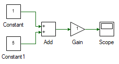
As seen, even though the order of evaluation was not explicitly mentioned by the user, there is an inherent sequence of execution for obtaining proper result and this sequence is determined automatically by the compiler. In the above case the task seems rather trivial but in most real world systems, the tools are interconnected rather deeply that the order cannot be established until a rigorous analysis has been carried out.
Another improtant simplification offered by model based design is the concepts of time conditional evaluvation. In most real world systems, different control models for the same system needs to be evaluated at different rates. For instance, a systems that actively monitors for faults and shuts the system down needs to be run at very high speed, a tool that reads input digital signal might have to be update every clock, while a tool that reads input ADC happens at much slower rate. For most application, updating control signal at a rate faster than the inputs to the system is a waste of computational resource. The ability of model based design to automatically figure out what is the optiomal update rate for each tool based on a wide range of factors makes it an extremely powerful yet simple solution compared to code based design.
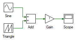
Consider the example shown below, where a Sine source which is updated every 2 ms is added to a Triangle Source updating every 3ms. The question of how fast the Adder needs to update is resolved by the compiler. If it was 2 ms, same as the first input, then the output does not instantly reflect changes to the second input. For instance, when second input updates at 3 ms, the adder output updates only at 4 ms. Similarly choosing the sample time of adder to be that of the second input does not work for the same reason. In this case, an update rate of 1 ms for the adder allows it to capture changes in both inputs faithfully. In most cases, this is not instantly decipherable.
In this section, the order in which Workbench evaluates the tools and the sample time it infers for each tool is explained in detail to give a better picture of what result is to expected. It must be noted that Workbench solves this complex task synchronously, i.e. as soon as any changes are made, the tool order and sample time are instantly computed even without having to run the model. This allows Workbench to report any errors or issue warnings based on this information instantaneously to the user, leading to a highly interactive environment, significantly cutting down on development time as well as reduce the hassle involed in debugging complex systems.
In most cases, before a tool is evaluated, its inputs are evaluated first. There are two exceptions to this rule, when a set of tools form a loop and, state-based tools whose outputs depends not its current inputs, but on its state/memory i.e., Discrete - Unit Delay is one such example where the output, equals the input from previous time step which is stored temporarily in its state/memory. Constrast this with Math Block - Elementary Function or Math Block/Continuous - Differentiator where output is a function of the current input. The order of tool evaluation for the system above, is shown below.
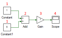
When two tools have the same order it means their order of evaluation does not matter, since their outputs at current time step is not a function of the output of tools that have the same order. It must be noted that this does not mean the tools that have same order are independent. Their outputs at current time step does not depend on one another's output at the current time step but may very well depend on values generated during previous time steps as would be the case in case of loops. In these cases where the order is the same, the compiler may choose to evaluate in certain order to minimize, branches due to different sample times, temporary variable etc.
Signal Sources are the only category of tools that have no input and has only output ports. Even though these have no inputs, their outputs are very much a function of current time step. All of these tool have a hidden input, the current simulation run-time. Hence these tools are always evaluated prior to non-state-based tools. State-based-tools are evaluated prior to both source tools as well as non-state-based tool since their output depends on neither's output at the current time step. The final ordering of the tool classes is given below:
State-based tools
Signal-sources
Non-state-based tools
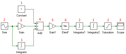
Withing the first category, if two state-based tools are connected to one another directly, the tool whose input is connected to another state-based tool is evaluated before the other one. This ensure that neither tool's state is affected prior to its output being updated. All signal-sources tools are of same evaluation order. Finally, all non-state-based tool's order is set to 1 greater than highest evaluation order of all the tools connected to its inputs. Tool evaluation order of a system containing all these tools is shown below.
The other special case in the determination of tool's evaluation order is when tools form loops. As mentioned earlier, for non-state-based tool, its evaluation order if a function of its input's evaluation order. In case of loops as shown below, this algorithm does not converge since output of every tool at current time step depends on every other tool's output at current time step. Due to this such a system is not allowed and will throw an Error EM0001 - Arithmetic loop. An example of such a system is shown beloww.

A loop is allowed and valid, if along every loop path there is at least one state-based tool present. Since these tools' order are not a function of its input, unless two or more of these are connected in tandem, they can act as starting point and ending point for tool evaluation order. Thus, the order always converges to a finitie value unlike the case of arithmetic loops. The same system considered earlier is cleared off its arithmetic loop error by simply adding a state-based tool such as Discrete - Unit Delay.

By default, all tool's inputs are read and outputs are updated, once every model step-time. In many cases, it may be desirable to evaluate and update certain sections of a model at a rate slower than the model step-time. In these cases, user must mention a sample time Ts, at which the tool must be evaluated. Workbench automatically infers and updates all the connected tool's Ts based on a number of factors.
There are three categories of sample time and based on the tool one or all of these may be supported:
Discrete
Continuous
Inherited
The sample time of a tool can be set in the Signal Attributes section of tool properties. If a tool's Ts is set as discrete, then a non-zero positive value greater than the smallest supported sample time of 1E-9 must be mentioned by the user. If the sample-time is smaller than this, including zero and negative values, then Warning WM0002 - Sample time smaller than least supported value is thrown. In these cases, the user set value is ignored and the tool's Ts is internally set to Continuous.
In addition to tool's Ts being set to Continuous when user mentioned sample time is less than least supported value, a tool can be manually set as continuously sampled. Some tools such as WSP_MB_LOT_MathBlockIntegrator, WSP_MB_LOT_MathBlockDifferentiator, etc., are permanently set to Continuous sample and cannot be changed by the user. When a tool is set as Continous, its inputs are read and outputs are updated at every simulation model step time, i.e. they are evaluated at every time step.
The final category within the possible sample time settings is Inherited sample time. Workbench estimates a tool's sample time when it's set to inherit based on a number of complex factors. Consider the simple case shown below which shall be analyzed for different sample time settings:

Sine's and Triangle's sample times are set to Discrete with Ts = 0.02 s and rest of the tools' sample times are set to Inherit:
In this case, the sample time of Add tool is inherited as 0.02 s because, if it were higher than 0.02 s then not all of the inputs samples would be captured and if it were lower then the adder block would be computing the same results multiple times unnecessarily because the inputs changes only every 0.02 s. By the sample logic, the sample time of all the blocks that follow Add is set to 0.02 s as well.
Sine's and Triangle's sample times are set to Discrete with Sine's Ts = 0.02 s and Triangle's Ts = 0.03 s, and rest of the tools' sample times are set to Inherit:
In this case, the sample time of Add tool is auto determined by the compiler to be 0.01 s. In this case, the greatest common divisor (gcd) is chosen, so that the output of the adder reflects any changes that might occur in either of the inputs.
If the gcd happens to be less than the smallest supported sample time of 1E-9 then Warning WM0002 - Sample time smaller than least supported value is thrown and the computed value is ignored and, the tool's sample time is set to Continuous. An example of this would be if in this case Triangle's sample time was 1/3 instead of 0.03 and Sine's was 0.02. The same would be the case, if the computed time was smaller than the model's step time with just the warning reported being different, Warning WM0001 - Tools sample time gcd too small.
In both the cases considered, the sample time was forward propagated, i.e. starting from source tools (has only output ports) and propagating towards sink tools (has only input ports). Next cases highlights a scenario where both forward as well as reverse propagation of sample time occurs.
Gain's sample time is set to Discrete with Ts = 0.05 s and the rest of the tools' sample times are set to Inherit:
Since the Gain's output is updated every 0.05 s, similar to previous cases, the Scope's sample time is inherited by forward propagation to be 0.05 s as well. The input to the Gain block has no user specified sample time. To achieve the best possible data resolution, the adder's sample time is inhertied by backward propagation to to 0.05 s as well and, the same is backward propagated so that the Sine and Triangle source tools are also updated at the same rate. It must be noted that if source and adder blocks where set to update at a faster rate, it would serve no purpose since the rate is limited by the Gain block's sample time setting.
Sine's and Triangle's sample times are set to Discrete with Ts = 0.03 s and Gain's sample time is set to Discrete with Ts = 0.02 s, and the rest of the tools' sample times are set to Inherit:
In this case, the Scope's sample time is inherted from Gain block to be 0.02 s. In case of Add block, there are conflicting sources of sample time. Forward propagation from Sine and Triangle would yield 0.03 s and backward propagation from Gain would yield 0.02 s. On first guess, one might assume choosing the gcd of 0.01 s, of the different sample times, would be the appropriate value. But on closer look it becomes evident that this choice is not the optimal value since the inputs change only every 0.03 s, updating output of adder at a faster rate yields no finer data points. Rather, the same result will end up being computed multiple times. Hence in this case, the Add tool's sample time is inherited to be 0.03 s.
Sine's sample time is set to Discrete with Ts = 0.03 s and Gain's sample time is set to Discrete with Ts = 0.05 s, and the rest of the tools' sample times are set to Inherit:
This is similar to the previous case with the difference being, the Triangle's sample time is set to Inherit. This minor difference completely alters the whole system's sample times. Same as before, Scope's sample time is inherited to be 0.05 s. But unlike the previous case, Add's sample time is inherited to be the gcd of input Sine's and output Gain's sample times, which equals gcd(0.03, 0.05) = 0.01 s. This is done so because, once the Add tool's sample time has be computed to be 0.01 s, this value is backward propagated to Triangle tool which inherites the same as its sample time. This allows for a faster update rate where the output of the adder will be of finer data resolution because one of the source itself is updating at a faster rate compared to previous case.
The above four simple cases discussed illustrates the core rules followed by the Workbench compiler to instantaneously compute all of the tools' sample times based on a few user set value. In summay, sample time of each tool set to Inherit is chosen to be the least possible such that the tool's output is not updated at a rate any faster than what is needed to capture all changes in all of its inputs. The sample time value, user set as well as inherited, can be observed in the tool's property.