Direct torque control of Induction motor

August 28, 2026
2 hours to complete
Workbench v1.5

Introduction

In this experiment, sensorless speed control of an induction motor using direct torque control (DTC) will be simulated. The dq motor model developed in the previous experiment will also be used. The estimator model and the switching algorithm will be modified to implement DTC. In addition to simulation, the controller will be evaluated on an actual induction motor in real-time.

Theoretical background

Motor model

The induction motor's stator-flux magnitude and position, electromagnetic torque, and speed are estimated from the stator voltages and currents as follows:

\frac{d\lambda _{s,\alpha \beta }}{dt} = V_{s,\alpha \beta } - R_{s}I_{s,\alpha \beta }\tag{1}

\theta _{s} = \tan^{-1}\left(\frac{\lambda _{s,\beta }}{\lambda _{s,\alpha }}\right)\tag{2}

\lambda _{s} = \sqrt{\lambda ^{2}_{s,\alpha } + \lambda ^{2}_{s,\beta }}\tag{3}

T_{\mathrm{em}} = \frac{2}{3}\times \frac{P}{2}(\lambda _{s,\alpha }I_{s,\beta } - \lambda _{s,\beta }I_{s,\alpha })\tag{4}

\lambda _{r,\alpha \beta } = \frac{L_{r}}{L_{m}}(\lambda _{s,\alpha \beta } - \sigma L_{s}I_{s,\alpha \beta })\tag{5}

\theta _{r} = \tan^{-1}\left(\frac{\lambda _{r,\beta }}{\lambda _{r,\alpha }}\right)\tag{6}

\lambda _{r} = \sqrt{\lambda ^{2}_{r,\alpha } + \lambda ^{2}_{r,\beta }}\tag{7}

\omega _{r} = \frac{d\theta _{r}}{dt}\tag{8}

\omega _{\mathrm{slip}} = \frac{3}{2}\times \frac{2}{P}\times R_{r}\times \frac{T_{\mathrm{em}}}{\lambda ^{2}_{r}}\tag{9}

\omega _{\mathrm{mech}} = \frac{2}{P}(\omega _{r} - \omega _{\mathrm{slip}})\tag{10}

where

V_s,αβ: stator voltage in the αβ frame
I_s,αβ: stator current in the αβ frame
λ_s,αβ: estimated stator flux linkage in the αβ frame
λ_s: magnitude of the estimated stator flux linkage
θ_s: angle of the estimated stator flux linkage with respect to the stator a-phase axis
λ_r,αβ: estimated rotor flux linkage in the αβ frame
λ_r: magnitude of the estimated rotor flux linkage
θ_r: angle of the estimated rotor flux linkage with respect to the stator a-phase axis
R_s: stator resistance
R_r: reflected rotor resistance
L_m: per-phase mutual inductance
L_s: L_ls + L_m, where L_ls is the stator leakage inductance
L_r: L_lr + L_m, where L_lr is the rotor leakage inductance
P: number of stator poles
T_em: estimated output/electromagnetic torque
ω_slip: estimated rotor electrical slip speed
ω_r: estimated speed of the rotor flux-linkage vector
ω_mech: estimated rotor mechanical speed
σ: leakage factor given by $\sigma = 1 - \frac{L^{2}_{m}}{L_{s}L_{r}}$

The αβ quantities are obtained from their corresponding abc quantities using the following equation:

\alpha \beta = a + b \times e^{j2\pi /3} + c \times e^{j4\pi /3}\tag{11}

This is the amplitude-invariant space-vector transform. The factor 2/3 in Eqn. 4 accounts for this scaling. Use a quadrant-aware arctangent when implementing Eqns. 2 and 6.

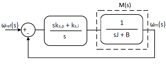
Once the mechanical speed ω_mech is estimated, the electromagnetic torque required to move the speed closer to the desired value can be obtained using a PI controller. The procedure for designing the controller is the same as that used in earlier experiments. The output of the speed-loop PI controller is the desired electromagnetic torque, T_em,ref. The system transfer function is shown below:

Speed loop PI controller

The inverter switching states for DTC are determined from the following three variables:

the error between the desired and estimated electromagnetic torque, $\delta T_{\mathrm{em}} = T_{em,\mathrm{ref}} - T_{\mathrm{em}}$
the error between the desired and estimated stator-flux-linkage magnitude, $\delta \lambda _{s} = \lambda _{s,\mathrm{ref}} - \lambda _{s}$
the current position of the stator-flux-linkage vector, $\theta _{s}$

The principle is that if the torque error is positive and the flux-linkage error is negative, the switching state is chosen so that the electromagnetic torque increases while the stator flux linkage decreases. For example, consider the case in which θ_s is between -π/3 and +π/3. Under this condition, the effect of each inverter switching state on the electromagnetic torque and stator flux linkage is given in the table:

Switch state			T_em	λ_s
A	B	C	T_em	λ_s
ON	OFF	OFF	Indeterminate	Indeterminate
ON	ON	OFF	Increase	Increase
OFF	ON	OFF	Increase	Decrease
OFF	ON	ON	Indeterminate	Indeterminate
OFF	OFF	ON	Decrease	Decrease
ON	OFF	ON	Decrease	Increase
ON	ON	ON	Decrease/Increase	No change
OFF	OFF	OFF	Decrease/Increase	No change

Similarly, the effect of each inverter switching state on T_em and λ_s can be determined for all values of θ_s, as illustrated in Reference 1. Applying a zero vector in the case above leads to a decrease in T_em if the speed is positive (counterclockwise) and an increase in T_em if the speed is negative. Of the eight switching combinations, only switching states that produce determinate effects are chosen to regulate motor torque and flux.

Simulation of induction motor speed control

The above speed control model is simulated using Workbench in this section.

Open Workbench and pin the Explorer and Properties docks.
Navigate to and open the IMDTCControl project file in the Experiment5\Simulation folder, usually found at C:\Program Files (x86)\Sciamble\WorkBench v1\Examples\CUSPLab\AdvancedDrives.
The script file computes the reference stator flux linkage at the rated operating condition using Eqns. 1 through 10. It also computes the speed PI-controller gains for a phase margin of 60° and a crossover frequency of 25 rad/s. Change these parameters as desired to test the motor under different conditions.
Open the model file:

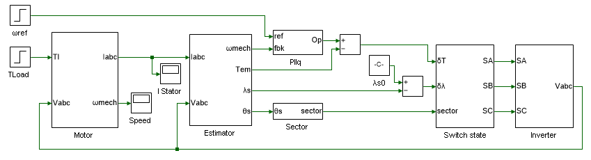
The leftmost section contains the induction motor dq model designed in the previous experiment. The electromagnetic torque, rotor mechanical speed, and stator flux linkage are estimated in the Estimator subsystem using Eqns. 1 through 10. The desired torque is obtained from the estimated speed and the desired reference speed using a PI controller, the output of which is the desired electromagnetic torque. The inverter switching states are determined in the Switch state subsystem based on the errors between the desired and estimated electromagnetic torque and stator flux linkage. Finally, these switching states are applied to the mathematical model of an ideal 3Φ inverter in the Inverter subsystem to obtain the terminal voltages applied to the induction motor.
Run the simulation model and observe the stator current, speed, and output torque.
Modify the PI-controller gain values to generate underdamped and overdamped responses. Rerun the simulation and verify the results.

Adjust the torque and flux hysteresis band within the Switch state subsystem to the values listed below and rerun the simulation.

Tool name	Property field	Property value	Comments
Hysteresis	Lower threshold	-IMParam:δλ * 2	Stator flux linkage hysteresis band.
Hysteresis	Hysteresis	Upper threshold	IMParam:δλ * 2	Stator flux linkage hysteresis band.
Hysteresis 1	Lower threshold	-IMParam:δTem * 2	Electromagnetic torque hysteresis band.
Hysteresis 1	Hysteresis 1	Upper threshold	IMParam:δTem * 2	Electromagnetic-torque hysteresis band.

Observe the current and speed results. Repeat the previous step while gradually increasing the band until the system becomes unstable.

This concludes the simulation of induction motor direct torque control. In the following section, a pre-built induction motor direct torque control model is run in real-time.

Real-time direct torque control of an induction motor

Open Workbench and pin the Explorer and Properties docks.
Navigate to and open the IMDTCControl project file in the Experiment5\Realtime folder, usually found at C:\Program Files (x86)\Sciamble\WorkBench v1\Examples\CUSPLab\AdvancedDrives.
Expand the project in the Explorer and open the ModelFile model file shown below:

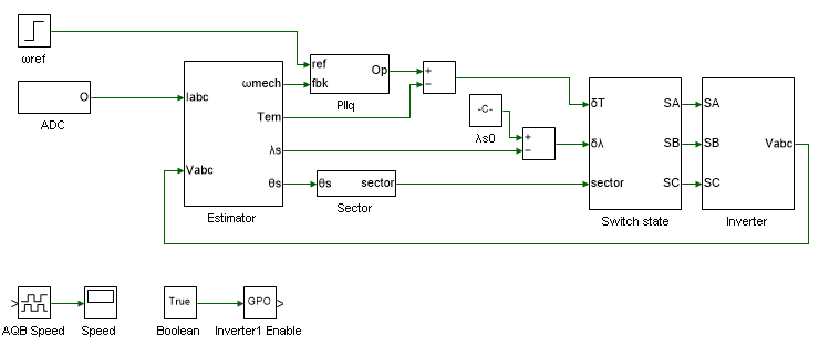
The model is the same as the one used in simulation, except that the induction-motor model has been replaced by stator currents measured from the actual motor. The estimator computes motor speed from the measured currents and commanded stator voltages; the separate encoder-speed scope is used only to observe and validate the estimate.
The Init() function in the IMParam script file computes the controller parameters from the motor parameters, loop crossover frequency, and phase margin. Set the speed-loop crossover frequency ωc and phase margin φm in the script to the same values used in simulation.
The Init() function must be called before running the simulation model to initialize the controller gain values. To do this, open the project properties, double-click the IMDTCControl project node in the Explorer, and set the Prerun Model/Function to IMParam:Init().

Similarly, set Start model/Function to ModelFile to run the model after parameter initialization.
Click the button to run the model in simulation mode. Using DataPeek, verify that the controller-gain parameters computed by the Init() function match the values computed earlier.
Turn ON the DC power supply and set the voltage to 40 V.
Ensure that the button on the top dock is pressed to enable real-time mode. Click the run button.
Observe the speed and current results in the scope. Click to focus the results. After about 5 s, stop data logging by clicking .
Turn OFF the DC power supply.
If necessary, repeat the experiment for different loop crossover frequencies and phase margins.
Turn OFF the DC power supply and disconnect all connections, including the USB cable.

Lab report and reading assignment

List the k_p and k_i values of the speed PI controller.
Attach plots of the 3φ stator currents and motor speed from the simulation.
The model does not employ zero switching states. Modify the simulation to include these states as well.
List all the switching states for all values of stator flux-linkage position and list their effect on the electromagnetic torque and the stator flux linkage magnitude.
Attach the motor speed from real-time.
If there are any performance differences between vector control (the previous experiment) and DTC, explain the cause.

Reference

"Analysis and Control of Electric Drives: Simulations and Laboratory Implementation," Ned Mohan and Siddharth Raju, Wiley Publication.