Induction motor V/f control

August 28, 2026
2 hours 30 minutes to complete
Workbench v1.5

Introduction

In an induction motor, it is preferable to maintain the air-gap flux at its rated value for a fast dynamic electromagnetic-torque response. This is achieved in V/f control, where the ratio of the applied terminal voltage to its frequency is held constant at the rated-condition value. The motor speed is controlled by adjusting the applied frequency while maintaining a constant V/f ratio. This experiment covers the design of a closed-loop V/f speed controller for an induction motor.

Theoretical background

Small signal motor model

From the previous experiment, the per-phase equivalent model of an induction motor, containing both the electrical and mechanical models, is as shown below:

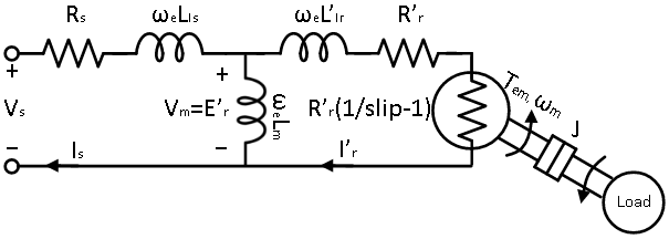
Linearized Induction motor electrical and mechanical model

In the steady-state per-phase equivalent circuit above, the s terms have been replaced by the complex variable jω. This is justified by the fact that the electrical time constants of practical induction motors are orders of magnitude lower than their mechanical time constants. Thus, when designing a controller for the motor's mechanical rotational speed, the transients associated with the motor's electromagnetic circuit can reasonably be ignored. Hence, the per-phase steady-state equivalent circuit can be assumed to be a sufficiently accurate model for deriving the motor's nonmechanical transfer function.

The air-gap flux is a function of the current flowing through the magnetizing inductance L_m, as given in Eqn. 1. If the voltage drops across the stator resistance R_s and stator leakage inductance L_ls are ignored, the voltage across the magnetizing inductance V_m equals the applied terminal voltage V_s, as given in Eqn. 2.

\Phi \propto I_{m} = \frac{V_{m}}{j\omega _{e}L_{m}}\tag{1}

I_{m} \approx \frac{V_{s}}{j\omega _{e}L_{m}}\tag{2}

where ω_e = 2πf, and f is the frequency, in hertz, of the applied terminal voltage. ω_e is related to the slip as follows:

\omega _{e} = \frac{P}{2} \times \omega _{\mathrm{sync}} = \frac{P}{2} \times (\omega _{\mathrm{mech}} + \omega _{\mathrm{slip}}) = \frac{P}{2} \times (\omega _{\mathrm{mech}} + \mathrm{slip} \times \omega _{\mathrm{sync}})\tag{3}

For a fast dynamic response, the flux is maintained at its rated value throughout most of the induction motor's operating region. Maintaining it above the rated value will lead to core saturation, increased losses, and harmonics. Maintaining it below the rated value will lead to increased rotor losses and will limit the maximum continuous torque that can be generated. Thus, under most operating conditions, the applied terminal voltage can be expressed as a function of the applied frequency:

V_{s} \approx \frac{V_{s, \mathrm{rated}}}{\omega _{e, \mathrm{rated}}} \times \omega _{e} = C \times \omega _{e}\tag{4}

where V_{s, rated} and ω_{e, rated} are the rated per-phase terminal voltage and frequency.

The motor speed is controlled by adjusting the frequency of the applied voltage using a PI controller. To tune this controller for the desired performance, a system transfer function linking the applied frequency to the rotor speed is derived in the following section.

The mechanical model of the induction motor is given in Eqn. 5. Under steady-state conditions, the torque generated by the motor, T_em, equals the sum of the load torque T_l and the torque required to compensate for frictional losses, T_fric. Under transient conditions, when T_em ≠ T_l + T_fric, the motor accelerates if the former is greater than the latter, storing the excess energy as inertial energy. It decelerates if the former is less than the latter, losing previously stored inertial energy. The motor inertia is identified as J in Eqn. 5, where ω_m is the mechanical rotor speed.

T_{\mathrm{em}} = T_{l} + T_{\mathrm{fric}} + J\frac{d\omega _{m}}{dt}\tag{5}

The frictional component arises from various factors and always opposes the direction of rotation. Of the many causes, only Coulomb friction, which is constant, and viscous friction, which varies proportionally with rotational speed, are considered because they have a significant effect on the steady state. The torque associated with Coulomb friction is denoted by T_c, and that associated with viscous friction is given by $B \times \omega _{m}$ , where B is the coefficient of viscous friction. Substituting these into Eqn. 5 yields the final mechanical model as given in Eqn. 6.

T_{\mathrm{em}} = T_{l} + T_{c} + B\omega _{m} + J\frac{d\omega _{m}}{dt}\tag{6}

which can be expressed in transfer function form as:

\frac{\omega _{m}(s)}{T_{\mathrm{em}}(s) - T_{l}(s)} = \frac{1}{sJ + B}\tag{7}

From the equation above, under constant-load conditions, a small incremental perturbation in electromagnetic torque, ΔT_em, leads to an incremental change in rotor speed, Δω_m:

\Delta \omega _{m}(s) = \frac{\Delta T_{\mathrm{em}}(s)}{sJ + B}\tag{8}

Having established the small-signal relationship between T_em and ω_m, the relationship between T_em and the applied frequency must be established to complete the system model. From the equivalent circuit, the output power of an induction motor is given by Eqn. 9. This is the same as the product of electromagnetic torque and motor speed.

P_{\mathrm{out}} = 3 \times I_{r}^{\prime 2} \times R'_{r} \times \frac{1 - \mathrm{slip}}{\mathrm{slip}}\tag{9}

T_{\mathrm{em}} = \frac{P_{\mathrm{out}}}{\omega _{m}} = \frac{P_{\mathrm{out}}}{(1 - \mathrm{slip}) \times \omega _{\mathrm{sync}}} = \frac{3 \times I_{r}^{\prime 2} \times R'_{r}}{\mathrm{slip} \times \omega _{\mathrm{sync}}}\tag{10}

where $\omega _{\mathrm{sync}} = \frac{2}{P}\omega _{e}$ and P is the number of poles.

The reflected rotor current transfer function I'_r(s) in the above equation equals:

I'_{r}(s) = \frac{V_{s}(s)}{Z_{s}(s) + \frac{Z_{m}(s)Z_{r}(s)}{Z_{m}(s) + Z_{r}(s)}} \times \frac{Z_{m}(s)}{Z_{m}(s) + Z_{r}(s)}\tag{11}

where

Z_{s}(s) = R_{s} + sL_{\mathrm{ls}}\tag{12}

Z_{r}(s) = \frac{R'_{r}}{\mathrm{slip}} + sL_{\mathrm{lr}}\tag{13}

Z_{m}(s) = sL_{m}\tag{14}

Under rated-load conditions, Z_m is much greater than Z_r, allowing the equation above to be simplified to Eqn. 15. Under light-load conditions, Z_r is much greater than Z_m and Z_s, allowing it to be simplified to Eqn. 16. To keep the PI-tuning method the same throughout the operating region, Z_s is added to the denominator of Eqn. 16 so that it matches Eqn. 15. This should not noticeably affect operation because, under light-load conditions, Z_s is much less than Z_r. These approximations do not significantly alter performance but reduce the order of the rotor-current-to-applied-stator-voltage transfer function, leading to a much simpler design.

I'_{r}(s) \approx \frac{V_{s}(s)}{Z_{s}(s) + Z_{r}(s)}\tag{15}

I'_{r}(s) \approx \frac{V_{s}(s)}{Z_{r}(s)}\tag{16}

Substituting this approximation into Eqn. 10 yields Eqn. 17.

T_{\mathrm{em}}(\mathrm{slip}) = 3 \times \frac{V_{s}^{2}}{\mathrm{slip} \times \omega _{\mathrm{sync}}} \times \frac{R'_{r}}{|Z_{s}(s) + Z_{r}(s)|^{2}}\tag{17}

Since V_s/ω_e is the constant C defined in Eqn. 4, the equation above becomes:

T_{\mathrm{em}}(\mathrm{slip}) = \frac{3C^{2}P^{2}\omega _{\mathrm{sync}}}{4\mathrm{slip}} \times \frac{R'_{r}}{|Z_{s}(s) + Z_{r}(s)|^{2}} = \frac{3C^{2}P^{2}\omega _{\mathrm{sync}}}{4\mathrm{slip}} \times \frac{R'_{r}}{|R_{s} + \frac{R'_{r}}{\mathrm{slip}} + j\omega _{e}(L_{\mathrm{ls}} + L'_{\mathrm{lr}})|^{2}}\tag{18}

\Rightarrow T_{\mathrm{em}}(\mathrm{slip}) = \frac{3C^{2}P^{2}\omega _{\mathrm{sync}}R'_{r} \times \mathrm{slip}}{4 \times |\mathrm{slip} \times (R_{s} + j\omega _{e}(L_{\mathrm{ls}} + L'_{\mathrm{lr}})) + R'_{r}|^{2}}\tag{19}

The system above is linearized around the rated operating condition. From the equation above, at the operating slip slip_op, a small incremental perturbation in slip, Δslip, leads to an incremental change in electromagnetic torque, ΔT_em:

\frac{\partial T_{\mathrm{em}}}{\partial \mathrm{slip}} = \frac{3C^{2}P^{2}\omega _{\mathrm{sync}}R'_{r} \times (R_{r}^{\prime 2} - (\mathrm{slip}_{\mathrm{op}}R)^{2})}{4 \times ((\mathrm{slip}_{\mathrm{op}}R)^{2} + 2\mathrm{slip}_{\mathrm{op}}R_{s}R'_{r} + R_{r}^{\prime 2})^{2}}\tag{20}

\frac{\partial T_{\mathrm{em}}}{\partial \mathrm{slip}} = k_{t}\tag{21}

where

R^{2} = R_{s}^{2} + (\omega _{e}L_{\mathrm{ls}} + \omega _{e}L'_{\mathrm{lr}})^{2}\tag{22}

PI Controller design

The overall transfer function is shown below, including the PI controller:

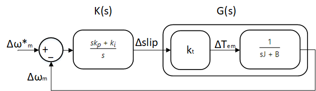
Induction motor small signal model

The overall open-loop transfer function is:

\frac{\Delta \omega _{m}(s)}{\Delta E_{s}(s)} = \frac{k_{s,p}s + k_{s,i}}{s} \times \frac{k_{t}}{Js + B}\tag{23}

where ΔE_s is the small-signal speed error applied to the PI controller.

The k_p and k_i values are chosen so that the crossover frequency ω of the transfer function above is ω_c, with a phase margin Φ = Φ_c. At the crossover frequency, the transfer function above has a magnitude of 1 and a phase angle of -π + Φ_c. This yields the following equation:

k_{s,p} = C2 \times k_{s,i}\tag{24}

where

C2 = \frac{1}{\omega _{s,c}} \times \tan\left(\Phi _{s} - \frac{\pi }{2} + \tan^{-1}\left(\frac{\omega _{s,c}J}{B}\right)\right)\tag{25}

and

k_{s,i}= \frac{\omega _{s,c}}{k_{t}}\sqrt{\frac{(\omega _{s,c}J)^{2} + B^{2}}{(\omega _{s,c} \times C2)^{2} + 1}}\tag{26}

Region of operation

The figure below shows the operating regions, i.e., the applied stator voltage as a function of frequency.

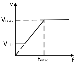
Induction motor V/f regions of operation

The system above was designed for the linear region. At low frequencies, the approximation V_m ≈ V_s fails because the voltage drop across the stator resistance is significant compared with the voltage drop across the magnetizing inductance. Consequently, applying the constant V/f ratio used in the linear region will not generate sufficient flux, and the electromagnetic torque is limited. To avoid this, at low frequencies, a constant minimum voltage is applied, until the linear region is entered.

At frequencies above the rated value, the V/f ratio can no longer be maintained because:

Exceeding rated voltage could cause motor insulation failure.
The available DC bus voltage is limited, hence the 3Φ inverter output voltage is limited.

Because of these limitations, above the rated frequency, the voltage is maintained at its rated value while the frequency is increased. This reduces the maximum torque because the air-gap flux is reduced. This is called field weakening, in which maximum electromagnetic torque is sacrificed to achieve higher speeds.

In the following section, a prebuilt closed-loop speed-control model is run in both simulation and real time.

Simulation of induction motor V/f control

Open Workbench and pin the Explorer and Properties docks.
Navigate to and open the IMabc project file in the Experiment3\Simulation folder, usually found at C:\Program Files (x86)\Sciamble\WorkBench v1\Examples\CUSPLab\AdvancedDrives.
Expand the project in the Explorer and open the IMabcModel model file shown below:

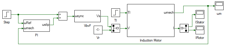
At the center of the model is a mathematical model of an induction motor. The system is modeled in the abc domain, and the details of its design are not covered in this experiment. The same model is developed in the dq domain as part of the next experiment. The inputs to the motor model are the 3Φ stator voltage and load torque. From these inputs, the model computes and outputs the 3Φ stator and rotor currents and the rotor's mechanical rotational speed. The load torque is simulated with a step of 0.05 N·m applied at 3 s. The 3Φ rotor voltages are set to 0 since the motor under consideration is a squirrel-cage induction motor, whose rotor is shorted. The 3Φ stator voltage is computed based on the desired input voltage frequency, inside the VbyF subsystem, using the V/f control discussed earlier.

The desired input-voltage frequency is, in turn, determined by the closed-loop speed controller. From the error between the desired and actual speeds, the PI controller determines the desired slip speed ω_slip. The frequency of the applied terminal stator voltage is determined by Eqn. 3, based on the desired rotor speed ω_mech and required slip speed ω_slip to achieve the desired rotor speed.
Open the IMParam script within the project in Explorer. A section of the file is shown below:
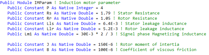
Update the motor parameter values in the script file to the values determined in the previous experiment.
The script file contains the function CalcKpKi(), which computes the speed controller's k_p and k_i gains from the motor parameters, controller phase margin, and crossover frequency. This is done using Eqns. 3 through 26. This function must be called before running the simulation model to initialize the controller gain values. To do this, open the project properties, double-click the IMabc project node in the Explorer, and set the Prerun Model/Function to IMParam:CalcKpKi() as shown below:

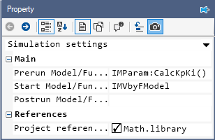
The crossover frequency ω_c is set to 50 rad/s, and the phase margin φ_c is set to 60° in the script file.
Similarly, set Start model/Function to IMabcModel, which is the V/f control model discussed earlier.

Note
The value set here is the model name, which is not always the same as the model's file name. The model name can differ from the file name displayed in the Explorer tab. It appears in the model properties, which can be viewed by double-clicking anywhere in the blank space of the model file.
Click the button to run the model.
Observe the motor-speed response to a step change in reference speed at 1 s and a step change in load torque at 3 s.
Make note of the k_p and k_i values. To do this, open the PI subsystem in the IMabcModel. Select the gain block labeled kp. Open the DataPeek dock on the right and select the button in the dock's toolbar to view the data of selected tool. The tool's gain value will be displayed as shown below:

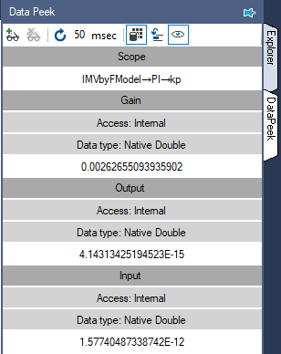
Similarly, select the tool labeled ki to look at the value of the integrator gain. The DataPeek can be used in a similar manner to view the runtime data of any tool.
Rerun the simulation for the following crossover frequencies: 20 rad/s, 100 rad/s, and 150 rad/s, and phase margins of 30, 60, and 90 degrees. Observe the speed and current responses for each of those values.

Note that the controller performs as expected only at and near the rated operating condition because the induction motor model was linearized in Eqn. 20 around this operating point. Also, during the derivation of the system equation, a major simplifying assumption was made, that the time constant of the mechanical system is much higher than that of the electrical system. This justified the use of the steady-state electrical per-phase equivalent motor model to derive the system transfer function. This assumption becomes increasingly invalid as the crossover frequency/bandwidth of the speed-control loop increases.

In the following section, closed-loop V/f speed control is implemented in real time to control the induction motor speed and observe the motor-speed and current responses under different load conditions and controller parameters.

Real-time V/f control of induction motor

Open a new Workbench session.
Create a new project and add a model file to it. Set this model file as the Start model/Function in project properties.
Open model properties and set the Step time to 0.0001 and the Run time to 5.
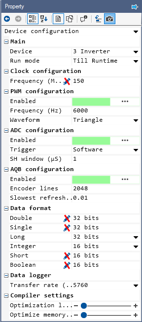
Within the project properties, select the drop-down menu on the top and select Device Configuration. Within this, change the following properties:
1. Change Device within the Main subdivision to 3 Inverter.
2. Change Run mode within the Main subdivision to Till Runtime.
3. Change Waveform within the PWM configuration subdivision to Triangle.
4. Change Encoder lines within the AQB configuration subdivision to 2048.
5. Change Transfer rate within the Data logger subdivision to 5760.
The overall model for real-time induction-motor V/f speed control is shown below. It will be built in the following steps.

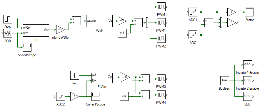
As in the previous experiment, a DC generator is used to load the induction motor. This is implemented using the tools in the bottom-left corner of the overall model shown above. To build this part of the model, drag the following tools from the Toolbox to the model and connect them as shown.

#	Tool type	Tool class	Tool name
1	Step	Signal Sources	Step
2	Analog Input	Hardware Integration	ADC
3	Gain	Math Block	Gain
4	Mag-Time Scope	Display	Scope
5	Subsystem	Signal Routing	Subsystem
6	Gain	Math Block	Gain1
7	Constant	Signal Sources	Constant
8	Adder Subtractor	Math Block	Add
9	Adder Subtractor	Math Block	Add1
10	PWM Output	Hardware Integration	PWM
11	PWM Output	Hardware Integration	PWM1

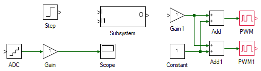
DC motor real-time current control model

While adding these tools, some of them might be highlighted in red. If the model has any such errors, the Numerical simulation and real-time prototyping Run button button is disabled until the errors are fixed. To determine the cause of an error, open the Messages tab at the bottom and select the Errors option. Clicking an error takes you to its source. These errors will be fixed in the following steps.

In the system above, the Step tool represents the desired DC-generator current and, in turn, the load torque. This is compared with the actual DC-generator current read by the ADC tool. The subsystem contains the PI controller that controls the applied terminal voltage to produce the desired current. The output of the subsystem is the terminal voltage. The following blocks convert this voltage to PWM duty cycles between 0 and 1.

Double-click the subsystem to open it and design the PI controller. Drag the following tools into the subsystem and connect them as shown:

#	Tool type	Tool class	Tool name
1	In-port	Signal Routing	I
2	In-port	Signal Routing	I1
3	Adder Subtractor	Math Block	Add
4	Gain	Math Block	Gain
5	Gain	Math Block	Gain1
6	Integrator	Math Block	Integrator
7	Adder Subtractor	Math Block	Add1
8	Saturation	Non-linear	Saturation
9	Out-port	Signal Routing	O

PI controller

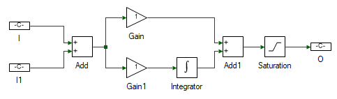
Change the properties of each tool within the subsystem to the values listed in the table below.

Tool name	Property field	Property value	Comments
I	Name	ref	PI controller reference.
I1	Name	fbk	PI controller feedback.
Add	Arithmetic operation	+-	Difference between the reference and feedback.
Gain	Gain	0.6132	DC motor PI current controller's proportional gain.
Gain1	Gain	250	DC motor PI current controller's integral gain.
Integrator	Integrator type	Anti-windup	This prevents the integrator from building up to a very large value due to real-world saturation.
	Integrator	Upper limit	15	Limits the maximum voltage output to the DC generator.
	Integrator	Lower limit	-15	Limits the minimum voltage output to the DC generator.
Saturation	Upper limit	15	Limits the maximum voltage output to the DC generator.
Saturation	Saturation	Lower limit	-15	Limits the minimum voltage output to the DC generator.
O	Name	Op	PI controller output. This is terminal voltage applied to the DC generator.

Change the properties of each tool outside the subsystem to the values listed in the table below.

Tool name	Property field	Property value	Comments
Step	Final value	0.5	A 0.5 A step change in DC-generator current. This translates to 0.05 N·m for the DC generator used.
Step	Step	Step time	3	Step the load at time 3 s.
ADC	Channel	5	Phase-A current of Inverter 2, to which the DC generator is connected.
Gain	Gain	5	Scaling to convert ADC signal to actual current. The scaling value is given within the ADC property.
Gain1	Gain	1/80	1/(2 x Vdc) to convert the voltage to a value between ±0.5.
Constant	Magnitude	0.5	Above signal is centered around 0.5 to get the duty cycle.
Add1	Arithmetic operation	-+	The duty cycle of one inverter leg is obtained by adding the scaled duty to 0.5, and that of the other leg is obtained by subtracting it from 0.5.
PWM	Channel	4	Each PWM channel controls the voltage across one of the output terminals.
PWM1	Channel	5	Each PWM channel controls the voltage across one of the output terminals.

Complete the remaining connections as shown:

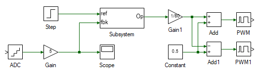
This completes the real-time design to emulate a step change in load torque.

In the following steps, a closed-loop V/f speed controller is designed using the tools in the top-left corner of the overall model shown earlier. To build the controller, drag the following tools into the model as shown:

#	Tool type	Tool class	Tool name
1	Step	Signal Sources	Step1
2	AQB Speed	Hardware Integration	AQB Speed
3	Mag-Time Scope	Display	Scope1
4	Gain	Math Block	Gain2
5	Adder Subtractor	Math Block	Add2
6	Subsystem	Signal Routing	Subsystem1
7	Gain	Math Block	Gain3
8	Constant	Signal Sources	Constant1
9	Adder Subtractor	Math Block	Add3
10	DeMux	Signal Routing	DeMux
11	PWM Output	Hardware Integration	PWM2
12	PWM Output	Hardware Integration	PWM3
13	PWM Output	Hardware Integration	PWM4

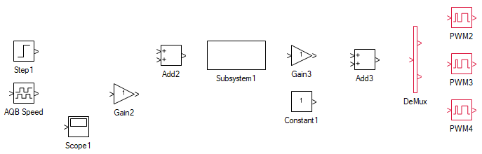
Induction motor real-time speed control model

The speed controller is the same PI controller that was designed for the DC-generator current controller in the previous steps. Copy and paste the PI-controller subsystem designed earlier (select the subsystem and press CtrlC, then CtrlV), as shown:

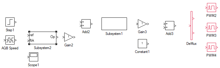
In the system above, the Step1 tool represents the desired induction-motor speed. This is compared with the actual induction-motor speed read by the AQB Speed tool. The output of the PI subsystem is the slip speed required to generate the desired steady-state motor speed. This is added to the desired motor speed to obtain the frequency of the applied motor terminal voltage. This is followed by a subsystem that contains the V/f logic and outputs the 3Φ induction-motor terminal voltage. The following blocks convert this voltage to PWM duty cycles between 0 and 1. Sine PWM modulation is used here.

Within the copy-pasted subsystem, set the following properties:

Tool name	Property field	Property value	Comments
Gain	Gain	k_p noted from the simulation for a crossover frequency of 50 rad/s and a phase margin of 60°.	Induction motor PI speed controller's proportional gain.
Gain1	Gain	k_i noted from the simulation for a crossover frequency of 50 rad/s and a phase margin of 60°.	Induction motor PI speed controller's integral gain.
Integrator	Integrator type	Anti-windup	This prevents the integrator from building up to a very large value due to real-world saturation.
	Integrator	Upper limit	0.1	Limited to the maximum slip of the induction motor.
	Integrator	Lower limit	-0.1	Limited to the minimum slip of the induction motor.
Saturation	Upper limit	0.1	Limited to the maximum slip of the induction motor.
Saturation	Saturation	Lower limit	-0.1	Limited to the minimum slip of the induction motor.

Open the V/f subsystem labeled Subsystem1. Drag the following tools into the subsystem and connect them as shown:

#	Tool type	Tool class	Tool name
1	In-port	Signal Routing	I
2	Gain	Math Block	Gain
3	Gain	Math Block	Gain1
4	Integrator	Math Block	Integrator
5	Increment	Math Block	Increment
6	Elementary Function	Math Block	Elementary Fnc
7	Multiplier Divider	Math Block	Multiply
8	Out-port	Signal Routing	O

V/f control subsystem

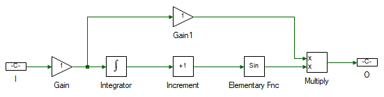
Change the properties of each tool within the subsystem to the values listed in the table below.

Tool name	Property field	Property value	Comments
I	Name	ωsync	Synchronous speed.
Gain	Gain	2	Scaled by P/2 to convert mechanical synchronous speed to electrical angular frequency. The motor has four poles, or two pole pairs.
Integrator	-	No change	Integrates the frequency to obtain the angle of the terminal voltage.
Gain1	Gain	0.06238	Scales the frequency by the V_{ph-peak,rated}/2πf_rated ratio to obtain the magnitude of the applied 3Φ terminal voltage. The motor is rated for a 24 V line-to-line RMS voltage at 50 Hz.
Increment	Offset	{0, -2π/3, -4π/3}	Offsets the angle by 2π/3 and 4π/3 to obtain the voltage angles of all three phases.
O	Name	Va	Applied 3Φ terminal voltage.

The remaining blocks, namely Elementary Fnc and Multiply, compute the 3Φ terminal voltage based on the angle and magnitude.

Change the properties of each tool outside the subsystem to the values listed in the table below.

Tool name	Property field	Property value	Comments
Step	Final value	100	Induction-motor reference speed of 100 rad/s.
Step	Step	Step time	1	Step the reference at time 1 s.
AQB Speed	Channel	1	This is the DSUB port to which the encoder is connected.
Scope1	Realtime log	Enabled	By default, scope only logs data in simulation. To log in real-time as well, it must be enabled.
Gain2	Gain	157.08	2πf_rated/(P/2), which converts per-unit slip to mechanical slip angular speed.
Gain3	Gain	1/80	1/(2 x Vdc) to convert the voltage to a value between ±0.5.
Constant1	Magnitude	0.5	The signal above is centered around 0.5 to obtain the duty cycle.
DeMux	Number of ports	3	Split the muxed 3Φ duty-cycle to individual phases.
PWM2	Channel	1	Phase-A.
PWM3	Channel	2	Phase-B.
PWM4	Channel	3	Phase-C.

Note

Use scopes in real-time mode judiciously. The bandwidth available for real-time data logging is limited, so the sample rate of each scope decreases as the number of scopes logging real-time data increases. To observe slowly varying signals, consider using other tools in the Display toolbox. Compared with a Scope, these tools log slowly, at intervals of approximately 200 ms, and therefore do not consume much bandwidth.

Connect the tools as shown:

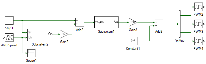
This completes the design of the closed-loop V/f induction-motor speed controller.

The final remaining components of the overall model are the current measurement at the top right and the inverter enable at the bottom right. Add the following tools and connect them as shown:

#	Tool type	Tool class	Tool name
1	Analog Input	Hardware Integration	ADC1
2	Analog Input	Hardware Integration	ADC2
3	Adder Subtractor	Math Block	Add4
4	Mux	Signal Routing	Mux
5	Gain	Math Block	Gain4
6	Gain	Math Block	Gain5
7	Mag-Time Scope	Display	Scope
8	True/False	Signal Sources	Boolean
9	Digital Output	Hardware Integration	GPO
10	Digital Output	Hardware Integration	GPO1
11	Digital Output	Hardware Integration	GPO2

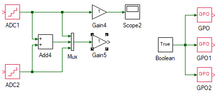
Current sensors and inverter enable

Set the properties of the above tools as given:

Tool name	Property field	Property value	Comments
ADC1	Channel	3	Inverter 1's/induction motor's phase-A current.
ADC2	Channel	4	Inverter 1's/induction motor's phase-C current.
Add4	Arithmetic operation	--	Negative sum of the phase-A and phase-C currents, i_b = -(i_a + i_c).
Mux	Number of ports	3	Mux the 3Φ currents.
Gain4	Gain	5	Scaling to convert ADC signal to actual current. The scaling value is given within the ADC property.
Gain5	Gain	5	Scaling to convert ADC signal to actual current. The scaling value is given within the ADC property.
Scope	Realtime log	Enabled	This scope is connected to measure only the phase-A current. It can instead be connected to Gain4 to measure the 3Φ currents, but the data logger does not have sufficient bandwidth to display three 50 Hz signals simultaneously with sufficient resolution.
Boolean		No change	Set to true to enable the inverter modules.
GPO	Channel	1	Enable inverter 1 which is connected to the induction motor.
GPO1	Channel	2	Enable inverter 2 which is connected to the DC generator.
GPO2	Channel	4	Controls the green LED on the side of the ThreeInverter module to indicate when the model is running in real time.

This completes the model for real-time, closed-loop V/f speed control of the induction motor.

Turn ON the DC power supply and set the voltage to 40 V.
Ensure that the button on the top dock is pressed to enter real-time mode. Click the run button.
Observe the speed and current results in the scope. Click to focus the results. After about 5 s, stop data logging by clicking .

Note
If the motor fails to reach the reference speed, stop the experiment and verify the controller gains, encoder feedback, wiring, and V/f calculation. Do not increase the V/f ratio above the motor's rated value.
Turn OFF the DC power supply.
If necessary, repeat the experiment for different controller gain values.
Turn OFF the DC power supply and disconnect all connections, including the USB cable.

Lab report and reading assignment

List the k_p and k_i values for the three different crossover frequencies and phase margins. Compare them with the values calculated by hand using Eqns. 3 through 26.
Attach plots of the motor-speed and 3Φ-current responses from the simulations for the three different crossover frequencies and phase margins. Comment on the differences in the responses and explain the reasons for them.
Attach plots of the motor-speed and phase-A-current responses from the real-time experiment.
If the motor is expected to perform as desired while operating at half its rating, how would the system be redesigned?
Read through the CalcKpKi() function and add comments to each line of code. Later experiments will require writing a script file to compute the controller parameters.