Introduction

• August 28, 2026
• 1 hour to complete
• Workbench v1.5
• • 
  • 

Introduction

Review, Safety considerations when working in power electronics, before proceeding.

There are three major components in the electric-drives system used to perform all the experiments in this course:

1. Three-inverter power module with on-board controller and data logger.

2. Coupled motor-generator system.

3. Workbench simulation and rapid prototyping software platform.

As an introduction to the Workbench-based electric-drives system described above, a prebuilt induction motor speed-control model will be simulated and run in real time. The following section gives a brief overview of the various components used to run the induction motor speed-control model. This will be followed by a simulation of the system in Workbench and its real-time implementation on the inverter-motor drive platform.

Overall system

The overall system is shown below and consists of the following components:

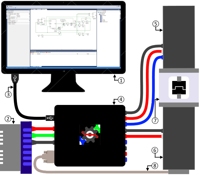
1. Workbench software platform: A numerical simulation platform that supports model and code-based design. A toolbox within the platform consists of various prebuilt, commonly used arithmetic, logical, conditional, and storage operators that can be used to model complex systems by dragging, dropping, and interconnecting these tools. In addition to simulating a system, the platform can generate digital-controller-specific code that can be programmed into a microcontroller or digital signal processor for real-time control.

2. Isolated DC power supply: This is used to power the inverter DC bus. In normal operation, the system is always run as a motor-generator pair, where energy transferred to the motor is mostly recuperated by the generator. Thus, the DC power supply only needs to supply the losses and the initial charging current.

   Note

   The communication channel between the computer and the three-inverter module is not isolated. Hence, the DC power supply must be electrically isolated to avoid common-mode current, which could otherwise potentially destroy the whole system.

3. USB A-B COM channel: Code and data transfer occur via USB 2.0. Under ideal conditions, the maximum data-transfer rate is 480 kbps, which translates to 15,000 samples per second for real-world variables such as motor currents, voltages, and speed.

4. Three 3Φ inverters: The hardware module contains all the power electronics, gate drivers, current and voltage sensors, digital signal processor, data logger, and programmer necessary for the design and deployment of common real-time motor-control algorithms. There are three 3Φ inverters, each rated at 50 V and 7 A. Forced cooling using two frame-mounted fans allows the inverters to be switched safely at up to 50 kHz under rated conditions. Each inverter is independently controlled by the onboard TI TMS320F28335 digital signal processor (DSP).

   In addition to providing PWM control of the inverters, the DSP reads feedback signals from the phase-A and phase-C current sensors of each 3Φ inverter, the DC-bus voltage sensor, the inverter overcurrent and overtemperature fault signals, and the motor-position encoder. The measured data, as well as other model variables, can be logged and viewed in real time on the Workbench software platform. This is made possible by a dedicated onboard data-transfer link between the computer and the DSP. The same channel is also used to transfer programs from the computer to the DSP.

5. Induction motor: The induction motor is rated at 24 V, 2.8 A continuous, and 1400 rpm at no load. In this experiment, the speed of this motor is maintained at a constant 100 rad/s regardless of load changes.

6. DC generator: The DC generator is rated at 60 V, 4 A continuous, and 4700 rpm at no load. It has an encoder mounted on the rear end of the rotor shaft to measure speed. Since the motor and generator are coupled, the magnitude of the generator's rotational speed is the same as that of the motor. The generator is used to emulate load changes.

7. Motor-generator coupler: The motor and generator are tightly coupled using an Oldham coupler. The coupling shaft is surrounded by a safety enclosure with viewing slots.

   Warning

   Do not leave loose objects nearby, as they can be pulled into the rotating motor shaft and flung at dangerously high speed. Always observe the system from a safe distance.

8. DSUB-15 encoder feedback: The motor/generator speed is measured using a 2048-line magnetic rotary A-quad-B encoder attached to the generator. This encoder contains 2048 evenly spaced, alternating north-south poles on a disc mounted on the rotor shaft. Two Hall-effect sensors are fixed to the motor frame. As the rotor turns, the alternating magnetic polarity generates voltage pulses at the sensor outputs. Counting the pulses per second yields the rotor speed. The sensors are positioned so that their output pulses are phase-shifted by 90°. The direction of rotation is obtained from the polarity of the phase shift between the two signals.

Induction motor speed control simulation

1. Copy the folder containing the prebuilt example project for this experiment, usually C:\Program Files (x86)\Sciamble\WorkBench v1\Examples\CUSPLab\AdvancedDrives\Experiment1, and paste it in a location where the user has permission to edit and save files, such as the Desktop folder.

2. Click the icon on the desktop to launch the application.

3. Workbench has tabs on the left, right, and bottom that represent docked windows, each of which displays information or provides controls for the user.

   

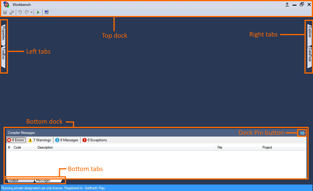
   Clicking these tabs reveals their respective docked windows. The content within these docks changes based on the context, as will be seen later.

4. Click the Toolbox tab in the left tab section and pin the window by clicking the icon in the upper-right corner. Similarly, pin the Explorer dock on the right. The tools in the Toolbox are grouped into categories based on their operation. Click the drop-down list, , to navigate between the tool classes.

5. Click the icon in the Toolbox dock to hide the toolbox for now.

6. The Explorer/Solution Explorer dock acts both as a file browser for navigating to, opening, adding, or removing project files and as a container that displays the project structure. The toolbar within the Explorer dock, , consists of the following buttons:

   1. : Creates a new project.

   2. : Opens an existing project.

   3. : Creates a new model or script file and adds it to the selected project.

   4. : Adds an existing model or script file to the selected project.

   5. : Removes the selected project, model, or script file. This does not delete it from the physical folder; it simply removes it from the current project.

   6. : Deletes the selected model or script file by sending it to the Recycle Bin.

   7. : Downloads project files.

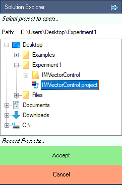
   Click the second icon, , to open an example project. This opens the file browser within the Explorer dock.

7. Navigate to the folder where the prebuilt example project was pasted in Step 1. Double-click the IMVectorControl.project node within that folder to open the project.

   

8. Click the icon to explore the files within the project. To display the model file, double-click the ModelFile node in the Explorer dock.

   

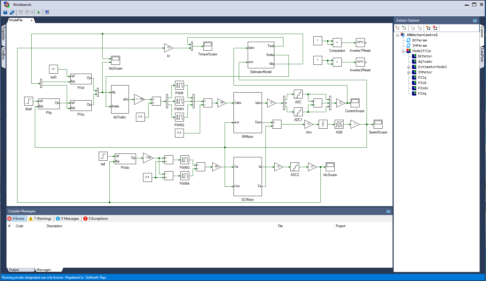
9. The details of this model will be explored in greater depth in later experiments. This experiment is solely meant to be an introduction to the system that will be used extensively in the following experiments. This system consists of a mathematical model of an induction motor subsystem labeled IMMotor. The motor voltage is modulated using Sine-PWM, the reference signal for which is derived from the inner current-loop and outer speed-loop PI controllers preceding it. The reference speed is stepped from 0 to 100 rad/s at time t = 1 s. The bottom section of the model contains the mathematical model of a DC motor. The motor is operated in torque-control mode, and its torque is stepped at time t = 3 s to emulate a sudden change in the load torque experienced by the induction motor. The aim of this experiment is to verify that the controller has been designed properly to compensate rapidly for the increased load demand and maintain the motor speed at the desired reference value.

10. Run the model by clicking the button in the top dock. Double-click the scope labeled SpeedScope to view the motor speed, which closely tracks the reference speed.

    

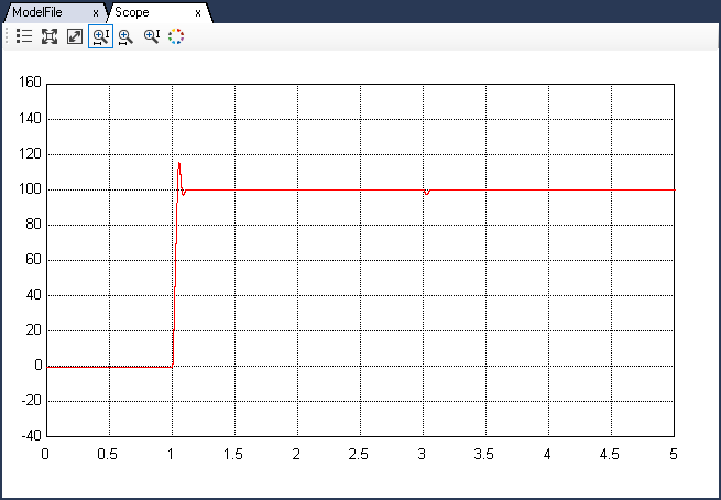
    To focus the data, double-click anywhere on the plot or click the button in the scope's toolbar. Also view the results in all other scopes in the model.

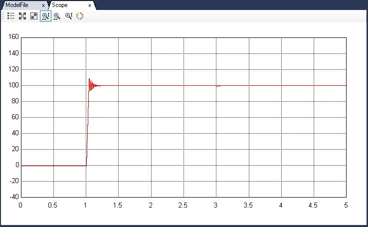
11. As shown above, the motor rotor speed closely matches the reference speed and settles quickly. Change this to a more underdamped response by changing the integrator gain in the PI block. To do this, double-click the PIIq subsystem in the MotorModel model file. Double-click the gain block labeled kI to open its properties in the Properties dock on the left. Multiply the Gain value by a factor of 10.

    

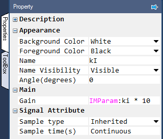
    Rerun the simulation and observe the speed result.

    

12. Change the kI gain to 0.1 times its original value, rerun the simulation, and observe the speed result.

13. Change the kI gain to 0.0001 times its original value, rerun the simulation, and observe the speed result.

This concludes the section on getting started with Workbench simulation. In the following section, the same model will be run in real time to control an actual induction motor.

Induction motor real-time speed control

1. Assemble the induction motor–DC generator set as shown below:

   

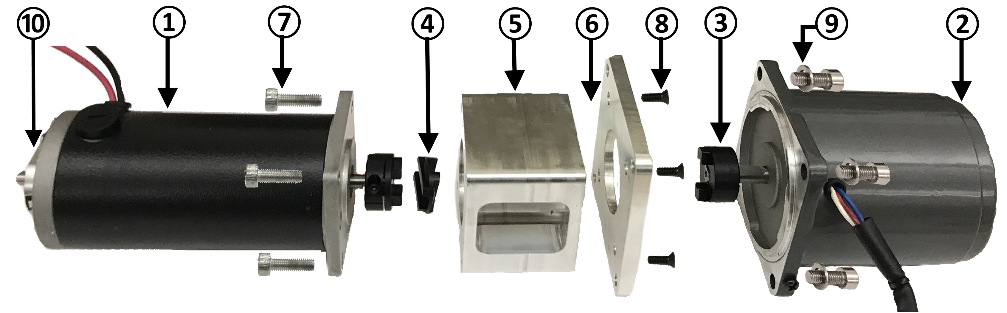
   1. DC Generator (one with A-quad-B encoder mounted on its back).

   2. Four-pole induction motor.

   3. Oldham coupler. Tighten if loose using M2.5 hex wrench.

   4. Oldham coupling disk. Attach it to the motor and generator coupling.

   5. Safety enclosure. The coupling unit resides inside the safety enclosure.

   6. NEMA 34 to NEMA 23 frame converter plate.

   7. M4 hex socket-head screws - x4.

   8. M4 hex flat-head/socket-head screws - x4.

   9. M5/M6 hex screws - x4.

   10. 2048-line A-quad-B encoder - Attach the encoder cable to the A-quad-B encoder.

2. The wiring color code followed is:

   DC (Inverter input):

   1. DC +ve - ● (Red)

   2. Ground - ● (Green)

   3. DC -ve  - ● (Black)

   
   

   AC (Inverter output):

   1. Phase A - ● (Black)

   2. Phase B - ● (Red)

   3. Phase C - ● (Blue)

   The inverter output terminals are located on the front panel of the three-inverter module. Connect the induction motor terminals to the Inverter 1 terminals so that the colors of the corresponding terminals match.

   Note

   The motor cable color might differ from the color of the banana terminal. In the following instructions, references to a motor-terminal color mean the color of the banana plug, not the cable.

   Connect the DC generator negative (-) (black terminal) to Inverter 2 A phase (black terminal) and DC generator positive (+) (red terminal) to Inverter 2 B phase (red terminal). The DC generator might have a third cable with a green terminal. This is the ground wire and must be left unconnected. Similarly, connect the DC power supply to the inverter input located on the back panel of the module.

   Warning

   Ensure that the DC power supply is turned off before making the connections. If the DC power supply does not have a dedicated ground terminal, that connection can be left floating. If present, it is strongly recommended that it be connected to the three-inverter module's ground terminal to mitigate any electrical hazard.

3. Connect the DSUB-15 terminal of the encoder cable connected to the generator to the Encoder 1 terminal on the back panel of the three-inverter module.

4. Connect one end of the USB cable (USB-A) to the computer and the other end (USB-B) to the back panel of the three-inverter module.

5. Turn ON the DC power supply and gradually ramp up the voltage from 0 to 40 V.

   Warning

   DC bus voltage must not exceed 42 V. A minimum of 20 V DC is needed to power the auxiliary power-converter inside the module. All the experiments have been designed with a DC bus voltage of 40 V unless mentioned otherwise.

6. Click the icon in the top dock of Workbench to transition from simulation mode, where the control algorithm was run on the computer using the linearized motor model, to real-time mode, where the control algorithm is executed in real time on a DSP and the generated signals are amplified to drive an actual motor. Workbench automatically identifies components that need to be evaluated in real time and automatically translates them into DSP-specific code.

   Note

   In real-time mode, the top dock changes from light blue to light salmon. In this mode, pressing Run immediately downloads the program to the connected real-time controller and begins execution. Any previously programmed code will be permanently overwritten. Take all necessary laboratory safety precautions.

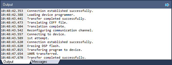
7. Click to run the control algorithm in real-time. The following message will be displayed if code has been transferred successfully:

   

8. Double-click SpeedScope to view the real-time result. Click the button in the scope's toolbar to fit the full simulation time along the X-axis. Press this button whenever the data goes out of focus. After about 5 s, stop data logging by clicking in the top dock. This stops only data logging. To power down the inverter, turn OFF the DC power supply and disconnect the USB cable to power down the controller.

   Note all other scope results as well. The 3Φ motor currents are not observed in real time because their frequency is too high for the limited-bandwidth data logger to capture enough data points.

This concludes the experiment. This experiment was a cursory introduction to concepts that will be revisited in subsequent experiments.

Lab report and reading assignment

1. Attach screenshots of the results from all scopes in the model in both simulation and real-time modes.

2. Explain the reason for the oscillatory behavior when the kI value is increased in the speed PI loop. Also explain why there is a steady-state error as kI → 0.

3. How would the induction motor speed and current plots differ if the load torque applied by the DC motor at t = 3 s were negative instead of positive, as used in this experiment?

4. Did the DC current reading on the power supply change when the induction motor was loaded by the DC motor? Explain why it did or did not.

5. Review the additional resource material on Workbench features available here.