
In this experiment, a dq model of a surface permanent-magnet AC (PMAC) motor will be simulated. The speed of the PMAC motor will be controlled using a closed-loop PI controller designed in this experiment. In addition to being simulated, the controller will be evaluated on an actual PMAC motor in real time.
Motor model
The following set of equations represents a linearized surface PMAC motor in the dq frame with the d-axis aligned with the rotor magnetic flux axis [1]:
where
Vsd, Vsq: stator d- and q-axis voltages, respectively
Isd, Isq: stator d- and q-axis currents, respectively
λfd: stator flux linkage due to the rotor magnets
Rs: stator resistance
Ls: Lls + Lm, where Lls is the stator leakage inductance and Lm is the per-phase mutual inductance
J: rotor inertia
B: coefficient of viscous friction
P: number of stator poles
Tem: output/electromagnetic torque
Tl: load torque
ωmech: rotor mechanical speed
ωm: d-axis rotational speed
Current controller design
Unlike in an induction motor, where the flux is established through the stator currents, the flux in a PMAC motor is established by the rotor magnets. Hence, under normal operating conditions, the d-axis current id is maintained at zero. Applying a negative id will cause the net air-gap flux magnitude to decrease because the flux induced by the stator d-axis current opposes the rotor-magnet flux with which the d-axis is aligned. The electromagnetic torque is adjusted by controlling the stator q-axis current. The desired stator dq currents are synthesized by controlling the applied stator dq voltages with a PI controller. The PI-controller gains are determined as in earlier experiments by defining the desired transient response of the system in terms of crossover frequency and phase margin.
To design the current PI controller, Eqns. 3 and 4 are substituted into Eqns. 1 and 2, and are rewritten in the following form:
The current-controller bandwidth is at least an order of magnitude higher than that of the outer speed controller. Hence, the d-axis speed ωm in the equations above can be considered constant and ignored in the small-signal analysis. Thus, the equation above can be rewritten in transfer-function form as:
The small-signal transfer function for the q-axis current and voltage is the same as the equation above. The overall current-loop transfer function is shown below.
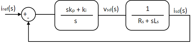
where
and
Speed controller design
The mechanical-system transfer function can be obtained from Eqn. 6. Ignoring the load torque as a disturbance:
Substituting Eqn. 5 into Eqn. 14:
The inner current loop can be modeled as a unity-gain transfer function. This assumption is valid as long as the response time of the inner current loop is an order of magnitude shorter than that of the outer speed loop. In other words, the crossover frequency of the inner current loop ωi,c >> the crossover frequency of the outer speed loop ωs,c. As with the current controller, the system above can be represented as follows:
The system above is similar to that of the current controller designed earlier. Following the same procedure, the speed-controller gains are:
where
and
where ks,p and ks,i are the proportional and integral gains, respectively, of the speed PI controller.
In this section, the speed-control model above is simulated using Workbench. The motor is assumed to be operating under steady-state conditions, and a step change in load torque is introduced at time t = 0.1 s. The resulting dynamic response is observed. Unlike in previous experiments, where the motor was simulated from a zero steady-state condition, the motor here is simulated from a nonzero steady-state condition. This greatly accelerates the simulation by allowing a larger step time because the changes in load torque, reference speed, and current are smaller than when starting from a zero steady-state condition.
Motor model design
Open-loop motor model
Create a new project and add a new model file and script file to it.
Set this model file as the Start model/Function in project properties.
Open the script file and initialize all the model parameters, as shown below, using the parameters estimated in the previous experiment.
Public Module PM

    Public Rs As Native Double = 0.7 / 2 ! Stator Resistance

    Public Ls As Native Double = 0.5E-3 / 2 ! Stator leakage inductance

    Public P As Native Double = 8 ! Number of Poles

    Public J As Native Double = 50E-6 ! Rotor Inertia

    Private ke As Native Double = 0.0416 / (2 * π) ! Back emf constant

    Public λf As Native Double = ke / (√2 / √3)


    ! Steady state operating condition

    Public f As Native Double = 60 ! Operating frequency

    Public ωmech0 As Native Double = f * 4 * π / P ! Rotor speed in rad/sec

    Private ωsync As Native Double = ωmech0 * P / 2 ! Electrical speed/ rotating flux speed

    Private Tem As Native Double = 0.1 ! Electromagnetic torque

    Public Tl0 As Native Double = Tem ! Load torque

    Public Isd0 As Native Double = 0 ! d axis current

    Public Isq0 As Native Double = Tem / ((P / 2) * λf) ! q axis current

    Public λsd0 As Native Double = Ls * Isd0 + λf ! d axis flux

    Public λsq0 As Native Double = Ls * Isq0 ! q axis flux

    Public Vsd0 As Native Double = Rs * Isd0 - ωsync * Ls * Isq0 ! d axis stator voltage

    Public Vsq0 As Native Double = Rs * Isq0 + ωsync * (Ls * Isd0 + λf) ! q axis stator voltage

    Public Vs0 As Native Double = (√2 / √3) * √(Vsd0² + Vsq0²) ! Peak stator phase voltage

    Public VPh0 As Native Double = Math:ATan2(Vsq0, Vsd0) * 180 / π !Initial stator voltage phase shift


    ! Speed PI Loop

    Private ωc As Native Double = 100 ! Cross over frequency

    Private φm As Native Double = 60 * π / 180 ! Phase margin

    Private ωcKpbyKi As Native Double = Math:Tan(φm)

    Private kt As Native Double = (P / 2) * λf ! torque constant

    Public ki As Native Double = ωc² * J / (kt * √(1 + (Math:Tan(φm))²)) ! Speed loop integrator gain

    Public kp As Native Double = ωcKpbyKi * ki / ωc ! Speed loop proportional gain


    ! Current PI Loop

    Private ωci As Native Double = ωc * 10 ! Cross over frequency, 10 times outer speed loop

    Private φmi As Native Double = φm ! Phase margin

    Private ωciKpibyKii As Native Double = Math:Tan(φmi - π / 2 + Math:Atan(ωci * Ls / Rs))

    Public kii As Native Double = ωci * √((Rs² + (ωci * Ls)²) / (ωciKpibyKii² + 1)) ! Current loop integrator gain

    Public kpi As Native Double = ωciKpibyKii * kii / ωci ! Current loop proportional gain

End Module
The first section of the script file sets the motor parameters obtained from the nameplate. These parameters can also be obtained by parameter estimation, as in TInv_AD_IMParameter. The following section calculates the steady-state currents and voltages for the motor operating at the rated speed and load torque, according to Eqns. 1 through 7. The next section calculates the PI gains of the outer speed controller using Eqns. 17 through 19 for a system crossover frequency of 100 rad/s and a phase margin of 60°. The final section computes the PI gains of the inner current controller using Eqns. 11 through 13 for a crossover frequency 10 times that of the outer speed loop and the same phase margin.
Open the model file and set its Step time property to 5E-5.
Set the Run time to 0.3.
Drag a Subsystem tool from the Signal Routing class in the Toolbox to the model.
Inside the subsystem, drag the following tools from the Toolbox and connect them as shown to create an abc-to-dq transformation.
| # | Tool type | Tool class | Tool name |
|---|---|---|---|
| 1 | In-port | Signal Routing | I |
| 2 | In-port | Signal Routing | I1 |
| 3 | Constant | Signal Sources | Constant |
| 4 | Adder Subtractor | Math Block | Add |
| 5 | Elementary Function | Math Block | ElemF |
| 6 | Elementary Function | Math Block | ElemF1 |
| 7 | Multiplier Divider | Math Block | Mul |
| 8 | Multiplier Divider | Math Block | Mul1 |
| 9 | Demux | Signal Routing | DeMux |
| 10 | Demux | Signal Routing | DeMux1 |
| 11 | Adder Subtractor | Math Block | Add1 |
| 12 | Adder Subtractor | Math Block | Add2 |
| 13 | Gain | Math Block | Gain |
| 14 | Gain | Math Block | Gain1 |
| 15 | Concatenate | Matrix Manipulation | Concat |
| 16 | Out-port | Signal Routing | O |
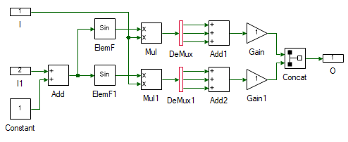
Change the properties of each tool to the values listed in the table below.
| Tool name | Property field | Property value | Comments |
|---|---|---|---|
| I | Name | abc | Input abc signal. |
| I1 | Name | theta | Input theta. |
| Constant | Magnitude | {0, 2 * π / 3, 4 * π / 3} | Muxed 3Φ phase shift signal. |
| Add | Arithmetic operation | +- | Add the cosine terms. |
| ElemF | Function | Cos | |
| ElemF1 | Function | Sin | |
| DeMux | Number of Ports | 3 | Splits the muxed signal into independent signals. |
| DeMux1 | Number of Ports | 3 | Splits the muxed signal into independent signals. |
| Add1 | Number of ports | 3 | Add the cosine terms. |
| Add2 | Number of ports | 3 | Add the sine terms. |
| Gain | Gain | √2 / √3 | Scale by sqrt(2/3). |
| Gain1 | Gain | -(√2) / √3 | Scale by -sqrt(2/3). |
| Concat | Pivot Dimension | 2 | Combines the signals to form a column matrix. |
| O | Name | dq | Output dq. |
Return to the main motor model by clicking its tab at the top.
Resize the subsystem so that all ports are visible. To resize a tool, drag any of the four squares at its corners.
Drag the following tools from the Toolbox to the model and connect them as shown to test whether the abc-to-dq transformation functions as expected.
| # | Tool type | Tool class | Tool name |
|---|---|---|---|
| 1 | Sine | Signal Sources | Sine |
| 2 | Constant | Signal Sources | Constant |
| 3 | Integrator | Math Block | Integrator |
| 4 | Mag-Time Scope | Display | Scope |
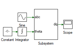
Change the properties of each tool to the values listed in the table below.
| Tool name | Property field | Property value | Comments |
|---|---|---|---|
| Sine | Phase shift (in degrees) | {0, -120, -240} | Input abc signal. |
| Constant | Magnitude | 2 * π * 1 | Frequency of the input signal in rad/s. |
| Integrator | Initial value | -π / 2 | The d-axis is aligned with the rotor flux. In the later steps, the d-axis angle is obtained by integrating the d-axis speed which is computed. For now, it is connected to a constant. |
Run the simulation and check whether the results are DC values, with the d-axis equal to zero and the q-axis positive.
Create a new subsystem. Drag the following tools from the Toolbox to the subsystem and connect them as shown to create a dq-to-abc transformation.
| # | Tool type | Tool class | Tool name |
|---|---|---|---|
| 1 | In-port | Signal Routing | I |
| 2 | In-port | Signal Routing | I1 |
| 3 | Constant | Signal Sources | Constant |
| 4 | Demux | Signal Routing | DeMux |
| 5 | Adder Subtractor | Math Block | Add |
| 6 | Elementary Function | Math Block | ElemF |
| 7 | Elementary Function | Math Block | ElemF1 |
| 8 | Multiplier Divider | Math Block | Mul |
| 9 | Multiplier Divider | Math Block | Mul1 |
| 10 | Adder Subtractor | Math Block | Add1 |
| 11 | Gain | Math Block | Gain |
| 12 | Out-port | Signal Routing | O |
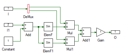
Change the properties of each tool to the values listed in the table below.
| Tool name | Property field | Property value | Comments |
|---|---|---|---|
| I | Name | dq | Input dq signal. |
| I1 | Name | theta | Input theta. |
| Constant | Magnitude | {0, 2 * π / 3, 4 * π / 3} | Muxed 3Φ phase shift signal. |
| Add1 | Arithmetic operation | +- | Add the cosine terms. |
| ElemF | Function | Cos | |
| ElemF1 | Function | Sin | |
| Add1 | Arithmetic operation | +- | Subtract the cosine and sine terms. |
| Gain | Gain | √2 / √3 | Scale by sqrt(2/3). |
| O | Name | abc | Output abc. |
Return to the main motor model by clicking its tab at the top.
Resize the subsystem so that all ports are visible. To resize a tool, drag any of the four squares at its corners.
Drag the following tools from the Toolbox to the model and connect them as shown to test whether the abc-to-dq transformation functions as expected. The output of ABCtoDQ is a column matrix, while the input of DQtoABC is a muxed signal. Therefore, the signal format must be converted.
| # | Tool type | Tool class | Tool name |
|---|---|---|---|
| 1 | Decatenate | Matrix Manipulation | Decat |
| 2 | Mux | Signal Routing | Mux |
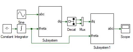
Change the properties of each tool to the values listed in the table below.
| Tool name | Property field | Property value | Comments |
|---|---|---|---|
| Decat | Pivot Dimension | 2 | Splits along the row. |
Run the simulation and check whether the results are the same as the input.
Delete the Decat and Mux tools.
The next step is to determine the motor's stator flux, as given in Eqn. 13. Create another subsystem, drag the tools listed below into it, and connect them as shown to implement the equation.
| # | Tool type | Tool class | Tool name |
|---|---|---|---|
| 1 | In-port | Signal Routing | I |
| 2 | In-port | Signal Routing | I1 |
| 3 | In-port | Signal Routing | I2 |
| 4 | Constant | Signal Sources | Constant |
| 5 | Multiplier Divider | Math Block | Mul |
| 6 | Multiplier Divider | Math Block | Mul1 |
| 7 | Gain | Math Block | Gain |
| 8 | Adder Subtractor | Math Block | Add |
| 9 | Integrator | Math Block | Integrator |
| 10 | Out-port | Signal Routing | O |
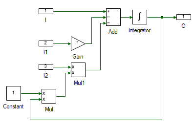
Change the properties of each tool to the values listed in the table below.
| Tool name | Property field | Property value | Comments |
|---|---|---|---|
| I | Name | vsdq | Stator voltage dq signal, vsdq. |
| I1 | Name | isdq | Stator current dq signal, isdq. |
| I2 | Name | wd | d-axis speed, ωd. |
| Gain | Gain | PM:Rs | Stator resistance, Rs. |
| Constant | Magnitude | [[0, -1], [1, 0]] | Rotational matrix. |
| Add | Number of ports | 3 | |
| Add | Arithmetic operation | +-- | |
| Integrator | Initial value | [[PM:λsd0], [PM:λsq0]] | Initial stator flux linkage. |
| O | Name | fsdq | Stator dq flux, λsdq. |
The next step is to determine the stator currents from the flux, as given in Eqns. 3 and 4. Drag the tools listed below into the model and connect them as shown to implement the equations.
| # | Tool type | Tool class | Tool name |
|---|---|---|---|
| 1 | Constant | Signal Sources | Constant1 |
| 2 | Adder Subtractor | Math Block | Add |
| 3 | Gain | Math Block | Gain |
| 4 | Decatenation | Matrix Manipulation | Decat |
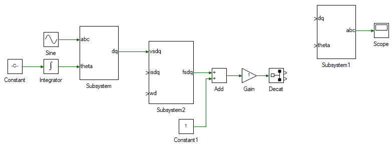
Change the properties of each tool to the values listed in the table below.
| Tool name | Property field | Property value | Comments |
|---|---|---|---|
| Constant1 | Magnitude | [[PM:λf],[0]] | Permanent-magnet flux vector [λfd, 0] in the rotor-aligned dq frame. |
| Add | Arithmetic operation | +- | Difference between stator and rotor flux. Eqns. 3 and 4. |
| Gain | Gain | 1/PM:Ls | Flux divided by stator inductance to obtain the stator dq currents. |
| Decat | Pivot Dimension | 2 | Split into isd and isq. |
Transfer the entire model designed so far into a subsystem. Select all tools and connections (CtrlA) and copy them (CtrlC). Delete the selection. Add a new subsystem to the blank model and paste the copied objects into it (CtrlV). This newly created subsystem represents the PMAC motor model.
The next step is to determine the motor speed to close the loop. In this simulation, viscous friction is neglected by setting B = 0, so Eqn. 6 reduces to J dωmech/dt = Tem - Tl. Add the following tools and connect them as shown.
| # | Tool type | Tool class | Tool name |
|---|---|---|---|
| 1 | Mux | Signal Routing | Mux |
| 2 | Gain | Math Block | Gain1 |
| 3 | Step | Signal Sources | Step |
| 4 | Adder Subtractor | Math Block | Add1 |
| 5 | Gain | Math Block | Gain2 |
| 6 | Integrator | Math Block | Integrator |
| 7 | Scope | Display | Scope1 |
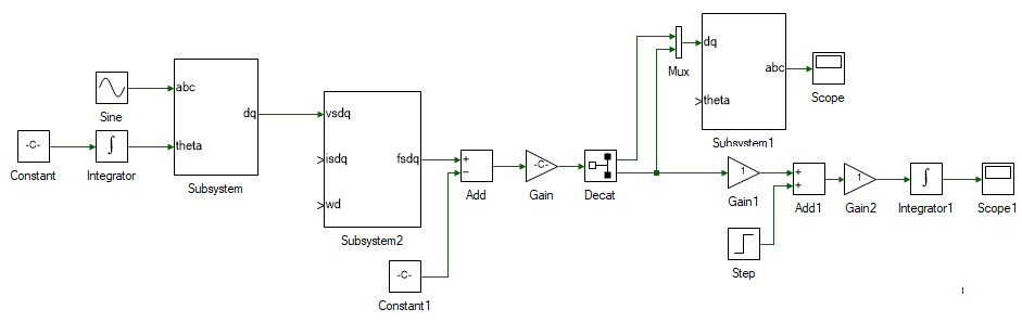
Change the properties of each tool to the values listed in the table below.
| Tool name | Property field | Property value | Comments |
|---|---|---|---|
| Gain1 | Gain | (PM:P / 2) * PM:λf | Eqn. 5. Tem calculation. |
| Step | Initial value | PM:Tl0 | Initial steady-state load torque. |
| Step | Final value | PM:Tl0 / 2 | Step change in load torque. |
| Step | Step time | 0.1 | Change load torque at time t = 0.1 s. |
| Add1 | Arithmetic operation | +- | Eqn. 6. Tem - Tl. |
| Gain2 | Gain | 1 / PM:J | Eqn. 6. |
| Integrator | Initial value | PM:ωmech0 | Eqn. 6, rotor mechanical speed calculation. |
All that remains is to close the loop. Delete the Constant tool connected to the abc → dq subsystem. This was initially used as the d-axis speed and is no longer needed because the actual d-axis speed, aligned with the rotor flux, is now available. Replace the Constant tool in the leftmost corner with a Gain tool, and set its Gain to PM:P / 2. This converts the rotor mechanical speed to the d-axis speed, as given by Eqn. 7. Connect the output of Integrator, which is ωmech, to the input of the newly added Gain block. The output of the Gain block is ωd. Connect it to the motor-flux subsystem. The output of Integrator connected to the newly added Gain block is θda, which must be connected to the theta input of the dq → abc subsystem. The stator dq currents for the stator-flux subsystem, isdq, are obtained by connecting the output of the Gain block, which is also the input of the Decat block. The overall PMAC-motor dq model, with its d-axis aligned with the permanent-magnet flux, is shown below.
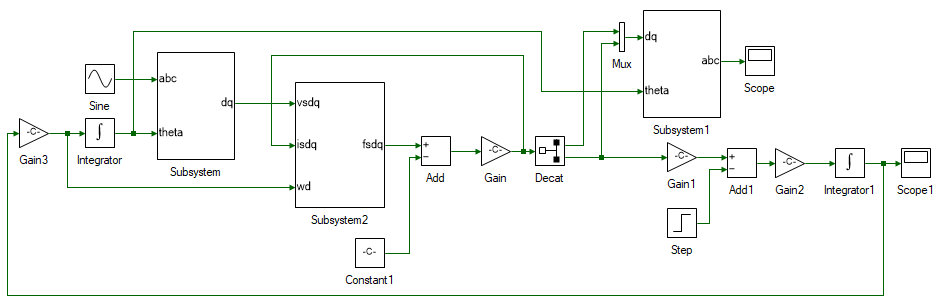
Set the stator 3φ voltage in the Sine block.
| Tool name | Property field | Property value | Comments |
|---|---|---|---|
| Sine | Magnitude | PM:Vs0 | Steady-state peak stator phase-voltage magnitude. |
| Sine | Phase shift (degrees) | {PM:Vph0, PM:Vph0 - 120, PM:Vph0 - 240} | Steady-state stator-voltage phase shift. |
| Sine | Frequency (Hz) | PM:f | Steady-state stator-voltage frequency. |
Add scopes to observe the abc and dq stator voltages and currents, motor speed, electromagnetic torque, and any other values of interest.
Run the simulation and observe the results.
This is the motor's response to a step change in load torque. The speed settles back to the synchronous speed even under open-loop conditions. If the load were increased rather than reduced, as in this case, the motor would become unstable. Change the Final value in the Step block to PM:Tl0 * 1.1, i.e., increase the load by 10%. Rerun the simulation and observe the results. The rotor quickly decelerates because the demanded torque exceeds the maximum electromagnetic torque that can be generated for the applied voltage. This is overcome by dynamically adjusting the applied voltage according to the load-torque demand using a PI controller, as shown in the following section.
If a runtime exception occurs, use the DataPeek window docked on the right to inspect each tool's inputs, outputs, and parameters immediately before the exception occurred.
This window can be used to observe the value of any tool or code variable at any time.
Click the  icon in the DataPeek window and select a tool to view its value.
Similarly, to view the value of a variable in the script file, place the cursor on the variable and double-click it. Its value will appear in the DataPeek window.
icon in the DataPeek window and select a tool to view its value.
Similarly, to view the value of a variable in the script file, place the cursor on the variable and double-click it. Its value will appear in the DataPeek window.
Motor current control
In this section, the current through the motor is controlled using a PI controller.
Within the motor-model subsystem, remove the Sine tool, replace it with an Inport, and name it Vabc. Similarly, remove the Step tool, replace it with an Inport, and name it Tl. These are the two inputs to the motor model. The outputs of the motor model are the stator currents and rotor mechanical speed. To bring these signals out of the subsystem, replace the Scope tool with an Outport tool and name it Iabc. Similarly, replace the Scope1 tool with an Outport tool and name it ωmech.
In the main model file, add a subsystem in which the d-axis PI current controller will be modeled. Double-click the subsystem to open it.
Drag the following tools from the Toolbox to the subsystem and connect them as shown.
| # | Tool type | Tool class | Tool name |
|---|---|---|---|
| 1 | In-port | Signal Routing | I |
| 2 | In-port | Signal Routing | I1 |
| 3 | Adder Subtractor | Math Block | Add |
| 4 | Gain | Math Block | Gain |
| 5 | Gain | Math Block | Gain1 |
| 6 | Integrator | Math Block | Integrator |
| 7 | Adder Subtractor | Math Block | Add2 |
| 8 | Saturation | Non-linear | Saturation |
| 9 | Out-port | Signal Routing | O |
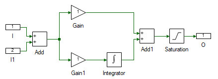
Change the properties of each tool to the values listed in the table below.
| Tool name | Property field | Property value | Comments |
|---|---|---|---|
| I | Name | Ref | Desired reference motor current. |
| I1 | Name | Fbk | Actual motor current. |
| Add | Arithmetic operation | +- | Difference between the desired and actual motor current. |
| Gain | Gain | PM:kpi | Current controller proportional gain. |
| Gain1 | Gain | PM:kii | Current controller integral gain. |
| Integrator | Integrator Type | Anti-windup | Reason explained later. |
| Integrator | Initial value | PM:Vsd0 | Steady-state stator d-axis voltage. |
| Integrator | Upper Limit | 20 | |
| Integrator | Lower Limit | -20 | |
| Saturation | Upper Limit | 20 | |
| Saturation | Lower Limit | -20 | |
| O | Name | Out | Applied terminal voltage to generate the desired current profile. |
When there is a large difference between the desired and actual currents, the PI controller produces a large output voltage to correct the error quickly. In a physical system, the magnitude of this voltage is limited by either the available DC-bus voltage or the voltage ratings of the motor and power electronics. Therefore, in a practical implementation of a PI controller, the controller output is limited to the maximum possible voltage. During transient conditions, when the actual current differs from the desired current, the integrator in the PI controller can rapidly build its output to a large value because of the persistent input error. When the error returns to zero, this large accumulated output does not immediately decay and can cause the actual current to overshoot the desired value. The error then becomes negative, causing the integrator output to fall, but it can fall by more than desired and cause the current to undershoot. This cycle can repeat, and the oscillation may decay slowly. To avoid this, the range over which the integrator is active is clamped by setting it to Anti-windup. If the integrator output reaches this limit, the integrator is disabled until the polarity of the error reverses. This improves the response of the system significantly.
Create a copy of the PI subsystem for q-axis current control.
Within the copied subsystem, set the Integrator's Initial value to PM:Vsq0.
The outputs of the PI controllers are dq voltages. These need to be converted to abc voltages before they are input to the motor model. To do this, copy and paste the dq-to-abc subsystem previously implemented within the motor model.
The output of the motor model consists of stator currents in the abc domain. To connect them to the PI current controllers' feedback inputs, they must be transformed into dq currents. To do this, copy and paste the abc-to-dq subsystem previously implemented within the motor model.
The overall current-controller system, after the addition of a few more tools listed in the following steps, is shown below:
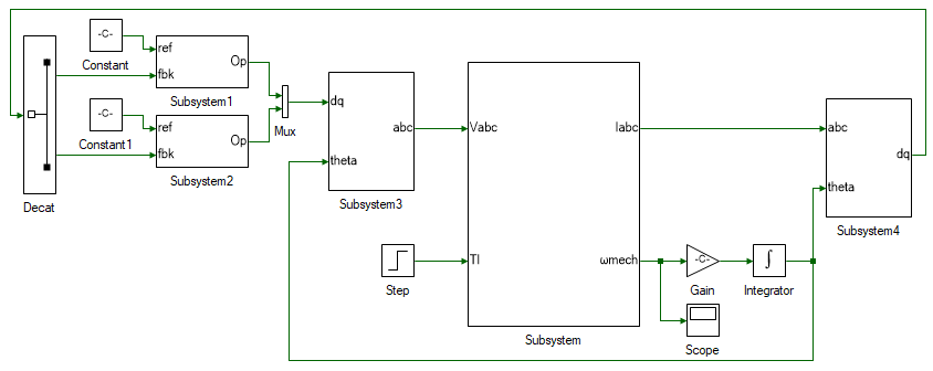
The motor model is within Subsystem. The d- and q-axis PI current controllers are within Subsystem1 and Subsystem2, respectively. The dq stator-voltage outputs of the PI controllers are converted to abc voltages using the dq-to-abc transformation within Subsystem3. Finally, the stator abc motor currents are converted to dq currents using the abc-to-dq transformation within Subsystem4.
Add the following tools and connect them as shown in the figure above:
| # | Tool type | Tool class | Tool name |
|---|---|---|---|
| 1 | Decat | Matrix manipulation | Decat |
| 2 | Constant | Signal Sources | Constant |
| 3 | Constant | Signal Sources | Constant1 |
| 4 | Mux | Signal Routing | Mux |
| 5 | Step | Signal Sources | Step |
| 6 | Gain | Math Block | Gain |
| 7 | Integrator | Math Block | Integrator |
| 8 | Scope | Display | Scope |
Change the properties of each tool to the values listed in the table below.
| Tool name | Property field | Property value | Comments |
|---|---|---|---|
| Decat | Pivot dimension | 2 | Split into isd and isq. |
| Constant | Magnitude | PM:Isd0 | Stator d-axis current, ideally set to 0 unless field weakening is used to increase the speed limit. |
| Constant1 | Magnitude | PM:Isq0 | Stator q-axis current. |
| Step | Initial value | PM:Tl0 | Initial steady-state load torque. |
| Step | Final value | PM:Tl0 / 2 | Step change in load torque. |
| Step | Step time | 0.1 | Change load torque at time t = 0.1 s. |
| Gain | Gain | PM:P / 2 | Eqn. 7. |
| Integrator | Initial value | -π / 2 | The d-axis is aligned with the rotor flux. In the later steps, the d-axis angle is obtained by integrating the d-axis speed which is computed. |
Run the simulation and observe the rotor speed. The rotor speed remains constant only as long as the load torque does not change. Once the load torque decreases, the rotor accelerates because the electromagnetic torque being produced is greater than the load torque. In reality, this will not occur, and the speed will settle because of either friction or the limited DC-bus voltage.
The current controller is applicable in systems where the torque is to be controlled directly. In applications where the rotor speed is to be controlled, the q-axis current PI controller is extended by adding an outer speed PI controller.
Motor speed control
In this section, the speed of the motor is controlled using a PI controller.
Replace the Constant1 block for the q-axis current reference with a PI-controller subsystem whose output will be the reference q-axis current.
Change the properties of the tools within the newly pasted PI controller to the values listed in the table:
| Tool name | Property field | Property value | Comments |
|---|---|---|---|
| Gain | Gain | PM:kp | Speed controller proportional gain. |
| Gain1 | Gain | PM:ki | Speed controller integral gain. |
| Integrator | Initial value | PM:Isq0 | Steady-state stator q-axis current. |
| Integrator | Upper Limit | 5 | Maximum stator current. |
| Integrator | Lower Limit | -5 | Minimum stator current. |
| Saturation | Upper Limit | 5 | Maximum stator current. |
| Saturation | Lower Limit | -5 | Minimum stator current. |
Connect the feedback input to the motor speed from the motor-model subsystem. Apply a constant-speed reference and set the Magnitude to PM:ωmech0. The overall system is shown below:
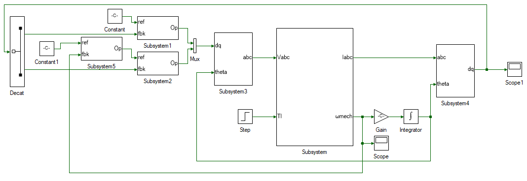
Run the simulation and observe whether the motor's steady-state speed matches the reference speed.
This concludes the simulation of PMAC motor vector control. In the following section, a prebuilt PMAC motor vector-control model is run in real time.
Assemble the PMAC motor-DC motor set as shown below:
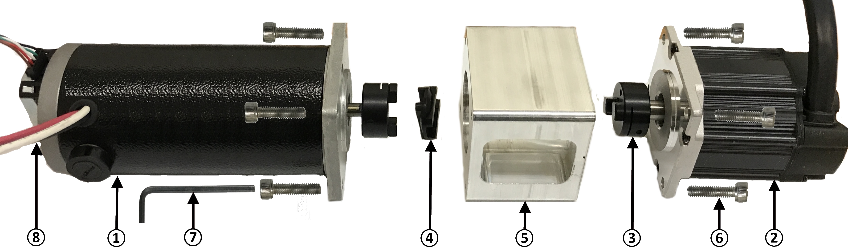
DC generator (the one with an A-quad-B encoder mounted on its back).
PMAC motor.
Oldham coupler. Tighten if loose using M2.5 hex wrench.
Oldham coupling disk. Attach it to the motor and generator coupling.
Safety enclosure. The coupling unit resides inside the safety enclosure.
M4 hex socket-head screws—eight.
M2.5 hex wrench—tighten the motor and generator to the safety enclosure.
2048-line A-quad-B encoder—attach the encoder cable to the A-quad-B encoder.
Connect the PMAC motor terminals to the Inverter 1 terminals, matching the terminal colors. Connect the DC generator's negative terminal (black) to phase A of Inverter 2 (black), and connect the DC generator's positive terminal (red) to phase B of Inverter 2 (red). Connect the encoder cable's DSUB-15 terminal to Encoder 1 on the back panel of the three-inverter module. Connect the DC power supply to the module's rear DC input, and connect the module to the computer with the USB cable.
 Warning
Ensure that the DC power supply is turned off before making the connections. If the DC power supply does not have a dedicated ground terminal, that connection can be left floating. If present, it is strongly recommended that it be connected to the three-inverter module's ground terminal to mitigate any electrical hazard.
Open Workbench and pin the Explorer and Properties docks.
Navigate to and open the PMVectorControl project file in the Experiment7\Realtime folder, usually located at C:\Program Files (x86)\Sciamble\WorkBench v1\Examples\CUSPLab\AdvancedDrives.
Expand the project and open the RotorInit model file shown below:
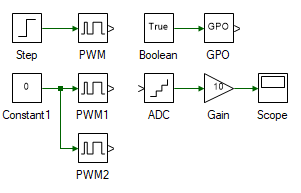
The incremental encoder does not output the rotor's actual absolute position. Instead, it outputs a pulse when the rotor turns through a certain angle. Because the initial rotor position cannot be determined using the incremental encoder, it is forcibly initialized to a predetermined position. This is achieved by briefly connecting the phase-A winding to Vdc and the phase-B and phase-C windings to 0, as implemented in the RotorInit model file. This ensures that the initial rotor magnetic-flux axis is aligned with the stator phase-A winding axis.
Open project properties and set the Start model/Function to RotorInit.
Turn ON the DC power supply and set the voltage to 40 V.
Ensure that the  button on the top dock is pressed to enter real-time mode. Click the
  button.
After about 5 s, click the  button to stop the model.
Open the ModelFile model file shown below:
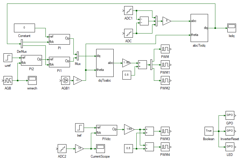
Return to the project properties and set Start model/Function to ModelFile before running the vector-control model.
The top section of the model contains the PMAC motor vector control and is a replication of the simulation model developed earlier, with a few additions to enable real-time control. On the left is the speed PI controller, followed by the d- and q-axis current PI controllers, whose outputs are the dq terminal voltages. The following subsystem converts the dq voltages to abc voltages. In the simulation model, this terminal-voltage signal was connected to the motor model. Here, it is converted to the inverter's PWM duty cycles and routed through the PWM tools to control the PMAC motor in real time. The PMAC motor model outputs the stator currents and rotor speed; a PMAC motor has no rotor-current output. In real-time mode, ADCs measure the actual motor stator currents, and the speed is measured using the actual motor's A-quad-B encoder. As with the PWM signal, the stator currents are routed through the ADC blocks, and the rotor speed is routed through the AQB block. This allows the same model to be run in both simulation and real time. During simulation, the tools from Hardware Integration act as 1:1 buffers and pass through all input signals. In real time, these tools read data from or write data to the real-time controller's peripherals.
The bottom section consists of the DC motor current control. This is used to emulate the load torque.
Turn ON the DC power supply and set the voltage to 40 V.
Ensure that the button on the top dock is pressed to enter real-time mode. Click the run button.
Observe the speed and current results in the scope. Click  to focus the results. After about 5 s, stop data logging by clicking .
Turn OFF the DC power supply.
If necessary, repeat the experiment for different loop crossover frequencies and phase margins.
Turn OFF the DC power supply and disconnect all connections, including the USB cable.
List the kp and ki values of the current and speed PI controllers.
Attach plots of the dq stator currents and rotor speed from the simulation without a controller, with the current controller, and with the speed controller, for both increasing and decreasing step changes in load torque.
In the simulated current-controller mode, if the coefficient of friction B in Eqn. 6 were 200E-6, at what speed would the rotor settle when the load torque was halved?
Design a PI controller to control the position of the rotor.
"Analysis and Control of Electric Drives: Simulations and Laboratory Implementation," Ned Mohan and Siddharth Raju, Wiley Publication.

