


A DC motor can be mathematically modeled as electrical and mechanical systems tied together by the relationships between back-emf and speed and between current and torque. In this experiment, the electrical and mechanical parameters of the DC motor are determined. These values are necessary to design a proper control system to control motor speed, torque, or position as will be seen in later experiments.
Motor model
Like all real-world systems, the DC motor exhibits nonlinear behavior. In the model shown below, a linearized DC motor model is considered for the sake of design simplicity. It will be verified in later experiments that the results from the simulated linearized model closely match those from the real-world motor, thus validating this approximation.
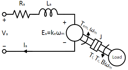
In a permanent magnet DC motor, such as the one used in this experiment, the stator contains the permanent magnet and the rotor contains the armature winding. When current flows through the armature winding, it generates flux, which interacts with the magnetic field established by the permanent magnet. This interaction generates an electromagnetic torque, Tem, which rotates or stalls the motor. The torque Tem is proportional to the armature current Ia as given in Eqn. 1 where kT is the torque constant.
As the motor rotates, the armature winding cuts through the magnetic field, which induces the back-emf Ea in the armature winding. As the motor rotates faster, the rate of change of magnetic flux dϕ/dt increases in proportion to the rotor speed. This is given by Eqn. 2 where ωm is the motor speed and ke is the back-emf constant.
The electrical power needed to drive the motor is given by \(E_{a} \times I_{a}\). The mechanical power needed to drive the motor is given by \(T_{\mathrm{em}} \times \omega _{m}\). Since these two quantities are the same (in SI units), Eqns. 1 and 2 give \(k_{t} = k_{e}\). Ra and La in the model above refer to the armature resistance and inductance, respectively. The voltage applied at the terminals, Va, equals the sum of the voltages across the passive elements—Ra and La—and the back-emf Ea. This represents the electrical model of the DC motor and is given in Eqn. 3, where Ea has been replaced with \(k_{e} \times \omega _{m}\) from Eqn. 2.
The mechanical model of the DC motor is given in Eqn. 4. Under steady-state conditions, the torque generated by the motor, Tem, equals the sum of the load torque Tl and the torque necessary to compensate for the frictional losses, Tfric. Under transient conditions, when Tem ≠ Tl + Tfric, the motor accelerates if the former is greater than the latter, storing the excess energy as inertial energy. It decelerates if the former is less than the latter, losing previously stored inertial energy. The motor inertia is identified as J in Eqn. 4.
The frictional component is due to various factors and always opposes the direction of rotation. Of the many causes, only Coulomb friction, which is constant, and viscous friction, which varies in proportion to the rotational speed, are considered because they have significant effects on steady-state operation. The torque associated with Coulomb friction is given by Tc, and that associated with viscous friction is given by \(B \times \omega _{m}\), where B is the coefficient of viscous friction. Substituting these into Eqn. 4 yields the final mechanical model as given in Eqn. 5.
Parameter estimation
In this experiment, the electrical model parameters Ra, La, and ke, and the mechanical model parameters Tc, B, and J, are determined for the DC motor as follows:
Ra: Use a multimeter. Alternatively, lock the rotor so that it does not rotate, apply a constant voltage Va of less than 2 V at the motor terminals, and measure the steady-state motor current Ia. Divide Va by Ia to obtain the armature resistance Ra. Locking the rotor eliminates the back-emf component in Eqn. 3, and the steady-state current eliminates the drop across armature inductance La. Thus, all the applied terminal voltage is dropped solely across the armature resistance.
La: As before, the rotor is locked to prevent it from rotating, thereby eliminating the back-emf component in Eqn. 3. The equation becomes:
When a step voltage of magnitude V is applied to the motor terminals at time t = tstep, the solution to the equation above for the current Ia is given in Eqn. 7. The derivative of Eqn. 7, evaluated at t = tstep, is given in Eqn. 8. Rearranging Eqn. 8 gives the armature inductance, as shown in Eqn. 9.
ke = kt: There are two ways to identify ke: one uses a coupled motor-generator set, and the other uses a single motor. In the former, run the generator at a constant speed while the motor terminals are left open. Measure the motor/generator speed ωm and the motor back-emf Ea, which is the same as the motor terminal voltage Vo because the terminals are open. From these two measurements, ke can be determined by using Eqn. 2.
Alternatively, if only a single motor is used, apply a constant voltage Vo at the motor terminals. Measure the motor current Ia and motor speed ωm at steady state. Compute ke from Eqn. 10, which is obtained from Eqn. 3, where the voltage drop across the inductance La is zero under steady-state conditions because Ia is constant.
The second method is used in this experiment because it is also used to estimate the frictional components, as explained in the next step.
Tc and B: If the motor is not accelerating, i.e., its speed is constant, and no load is connected, the inertial-torque and load-torque components in Eqn. 5 become zero, leading to the following equation:
Apply a constant voltage Vo at the motor terminals. Measure the motor speed ωm and current Ia. The electromagnetic torque Tem can be computed from the measured current Ia using Eqn. 1. Repeat the same process for different voltages and plot Tem (y-axis) versus ωm (x-axis). The resulting plot will be linear. The slope of the plot equals the coefficient of viscous friction B, and the y-axis intercept is the frictional torque Tc due to Coulomb friction.
J: Apply a constant voltage Vo at the motor terminals. Once the speed settles, measure the speed ωm and motor current Ia. At steady state, the electromagnetic torque Tem (Eqn. 1) solely compensates for drag due to friction. Disable the inverter so that the motor current dies down to zero rapidly. After this, there is no electromagnetic torque, and all the frictional losses must be supplied by the inertial energy. This causes the motor to stop gradually. This is summarized in Eqn. 12, which is obtained by setting Tem and the load torque Tl in Eqn. 4 to zero.
At the moment the inverter is disabled, at time t = Tdis, the frictional-torque component Tfric is the same as the electromagnetic torque Tem just before the inverter is disabled, and it can be obtained from the steady-state current Ia before disabling the inverter using Eqn. 1. Substituting this into Eqn. 12 yields:
 Note
NoteDisabling the inverter is not the same as setting the output voltage to 0. In the former case, the motor current extinguishes much faster than the motor speed decreases. After this point, the inertial energy is not lost in the armature resistance or returned to the source. If the terminal voltage were set to zero, the inertial energy, in addition to being lost through friction, would also be lost in the armature resistance because the back-emf would source current while the terminals were effectively shorted.
Ra: Measure across the motor terminals using a multimeter.
La:
Open Workbench and pin the Explorer and Properties docks.
Navigate to and open the DCMotor project file in the Experiment3 folder, usually found in the following location: C:\Program Files (x86)\Sciamble\WorkBench v1\Examples\CUSPLab\BasicDrives.
Expand the project and open the LsEstimate model file by double-clicking the model node. Open the model properties by double-clicking anywhere in the blank space of the open model. Copy the value in the property labeled Name, which if previously unchanged will be LsEstimate.
Since this project has more than one model file, the project must be told which model to run. To do this, open the project properties by double-clicking the project node in the Explorer dock, and paste the copied model name (LsEstimate) into the Start model/Function field.
Shown below is the LsEstimate model:
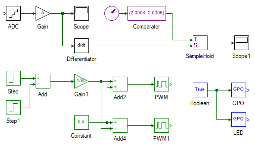
The GPO tool, among the components highlighted in blue in the bottom-right corner, is the Inverter 1 enable pin and is set to ON (True). The LED tool in the same section represents the green LED on the side of the three- inverter module, next to the red power LED. It is an indicator that glows when the code begins to execute. The tools highlighted in green represent the inverter PWM-generation logic, as seen in the previous experiment. For estimating inductance, the rotor must not rotate. Since it is rather difficult to physically lock the rotor from rotating, we instead excite it for a brief period. The excitation pulse is applied at time t = 2 s and has a magnitude of 40 V and a duration of 1 ms. During this brief interval, the motor does not develop sufficient electromagnetic torque to overcome the static friction, so the speed remains at zero, which has the same effect as locking the rotor.
As discussed above, the terminal voltage Vo and the current derivative I'a at t = 2 s, i.e., immediately after the armature winding is excited, are needed to estimate La. The simulation model is run at a step time of 0.2 ms. Even though this update rate is good enough for observing I'a, the rate at which the data itself is logged is much slower. Data from each evaluation is not logged to the computer because of the limited data-transfer bandwidth. Hence, simply adding a scope to observe I'a will, in most cases, not capture the data at the exact instant needed. This limitation is overcome by the blocks shown in purple. These capture I'a during the short interval between 2.0004 and 2.0006 s, immediately after the motor is excited, and hold it using a sample-and-hold block, which ensures that the sampled data is definitely logged to the scope.
Finally, among the blocks highlighted in black, the ADC block represents the motor-current feedback. Double-click it to view its properties and note the property labeled Signal Scaling. The inverse of this value represents the factor by which the ADC output must be scaled to obtain the actual current. The Gain block following the ADC block does this scaling.
Connect the motor (the one without the encoder) to Inverter 1 (the color of each motor terminal must match that of the corresponding inverter terminal). Even though the generator (the one with the encoder) is not used in this case, connect it to Inverter 2 instead of leaving the terminals open (once again, the color of each motor terminal must match that of the corresponding inverter terminal).
Connect the three-inverter module to the DC power supply. Connect the three-inverter to the computer via USB. Connect the generator speed feedback to the three-inverter's Encoder 1 DSUB connector in the back panel.
Turn ON the DC power supply and set the voltage to 40 V.
Ensure that the  button on the top dock is pressed to enable real-time mode. Click the run button.
Double-click the scope named Scope1 to view the data log of the Ia derivative. After about 5 s, when a step change is observed in the plot, stop data logging by clicking the  button. Automatically focus the scope result by clicking
  in the scope's toolbar. The result should look like the waveform shown below:
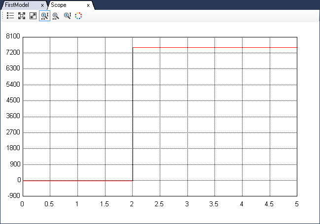
Zoom in and note the plot's peak, which is the Ia derivative immediately after the voltage pulse is applied to the motor.
Repeat the previous two steps to obtain at least five different readings.
Compute the value of La for each reading using Eqn. 9, where Va(tstep) = 40 V.
The motor armature inductance La is the average of these samples.
Close the LsEstimate model.
ke = kt, Tc, and B:
All three parameters are estimated using the same method in this step.
Open the keEstimate model within the same project.
Open the model properties by double-clicking the blank space, and copy the Name property.
Go to the project properties by double-clicking the project node, and set Start model/Function to the copied value.
The model is shown below. The motor is given a constant step voltage and the motor current and speed are measured.
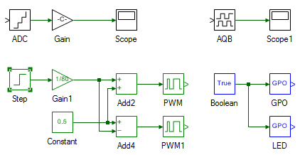
Open the Step tool's properties and set the Final value property to 10.
Ensure that the motor is connected as it was while estimating La and that the DC power supply is turned ON and set to 40 V.
Click , followed by  , to run the model in real time.
After about 5 s, when Scope1 has logged the data, click to stop data logging.
NoteThe motor will continue to run since only data logging was halted.
Record the results in a table with the following layout:
| Va (V) | Ia (A) | ωm (rad/s) | ke | Tem (Nm) |
|---|---|---|---|---|
where Va is the motor terminal voltage, which can be obtained from the Final value property of the Step block; Ia is the motor current logged in Scope; and ωm is the motor speed logged in Scope1. All these values must be measured after the motor reaches steady state following the application of the desired voltage. The remaining table entries are computed from these values and will be explained in the following steps. If any of the measured values are negative (due to sensor orientation), use the absolute value for the table.
Repeat the previous three steps for different motor terminal voltages from 10 V to 20 V in steps of 2 V. The voltage can be changed using the Step tool's Final value property.
Turn OFF the DC power supply and unplug the USB cable.
From the above table, ke, which is equal to kt, is computed using Eqn. 10. The final ke is the average of all the computed values.
Using the average kt, compute Tem for each Ia. Plot Tem (y-axis) versus ωm (x-axis).
Measure the slope of the plot to estimate the coefficient of viscous friction B, and use the y-axis intercept to estimate the frictional torque due to Coulomb friction Tc.
Close the keEstimate model.
J:
Open the JEstimate model within the same project.
Open the model properties by double-clicking the blank space, and copy the Name property.
Go to the project properties by double-clicking the project node, and set Start model/Function to the copied value.
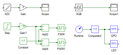
The model is shown below. The motor is given a step voltage of 25 V (the Step tool's Final value property) at t = 1 s. Once the motor has reached steady state, the inverter is disabled at t = 3 s. This places the inverter terminals at high impedance so that the inertial energy is lost only through friction.
Reconnect the USB cable and turn on the DC power supply.
Ensure that is pressed. Click to run the model in real time.
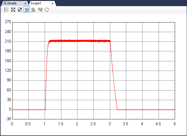
Open Scope1 to observe the motor speed. After data has been logged for 5 s, click to stop data logging. The results in Scope and Scope1 will look like this:
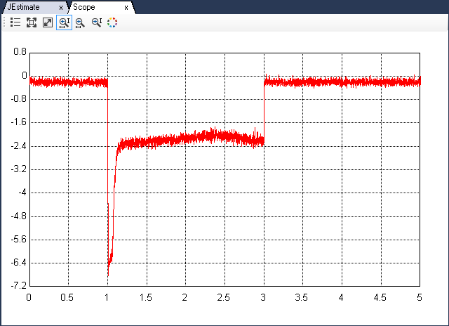
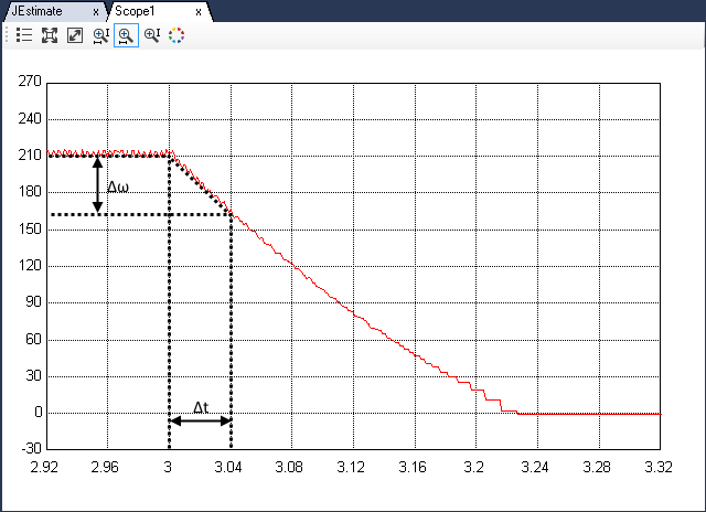
Zoom in on the speed at t = 3 s and determine the slope, as shown below.
In the current plot, note the current's magnitude just before the inverter is disabled at t = 3 s.
Calculate the inertia J using Eqn. 13. Use the absolute value of the steady-state current and the magnitude of the deceleration slope.
Turn OFF the DC power supply and disconnect all the connections including the USB.
This concludes the experiment on DC motor characterization. The parameters estimated in this experiment will be used in the following experiments to tune a PI loop that controls the motor speed.
Attach a plot of I'a from the La estimation.
Attach plots of Ia and ωm for different values of Va from the ke estimation.
Attach plots of Ia and ωm from the J estimation.
Attach the table from ke estimation.
List the results of all final parameter values.