Torque-speed characteristic and speed control of Induction motor

August 28, 2026
1 hour to complete
Workbench v1.5

Introduction

In this experiment, the open-loop torque-speed characteristic of an induction motor will be measured. As will be seen, the motor speed does not remain constant and tends to drop linearly with increasing load torque. The torque-speed characteristic will then be measured under closed-loop V/f-based speed control.

Theoretical background

At a fixed stator frequency and within the normal low-slip operating region, the induction motor's electromagnetic torque is approximately proportional to the slip and the square of the magnetizing current:

T_{\mathrm{em}} \propto s \times I_{m}^{2}\tag{1}

The magnitude of the magnetizing current can be approximated from the equivalent circuit developed in the previous experiment as:

I_{m} = \frac{V_{m}}{2\pi f \times L_{m}}\tag{2}

where V_m is the voltage across the magnetizing inductance, f is the frequency of the applied stator voltage, and L_m is the magnetizing inductance.

Slip s is a function of the number of motor poles P and the mechanical speed ω_mech, as given below:

\omega _{\mathrm{sync}} = \frac{2}{P} \times 2\pi f\tag{3}

s = \frac{\omega _{\mathrm{sync}} - \omega _{\mathrm{mech}}}{\omega _{\mathrm{sync}}}\tag{4}

If the stator leakage inductance and stator resistance are negligible, the voltage across the magnetizing inductance, V_m, is the same as the applied stator voltage V_s.

I_{m} = \frac{V_{s}}{2\pi f \times L_{m}}\tag{5}

Throughout motor operation, I_m is maintained at its maximum rated value, given by:

I_{m,\mathrm{rated}} = \frac{V_{s,\mathrm{rated}}}{2\pi f_{\mathrm{rated}} \times L_{m}}\tag{6}

This ensures that the maximum torque is produced for a given slip. If this value is maintained below its rated value, the motor's dynamic response and the maximum load torque that it can handle before stalling are reduced. If it is maintained above its rated value, the motor enters significant magnetic saturation, leading to lower-order torque pulsations, higher losses, and other effects that significantly impair motor operation. Thus, for all other operating frequencies, the voltage is maintained so that the ratio of voltage to frequency is the same as the ratio of rated voltage to rated frequency. This ensures that the rated magnetizing current flows through the motor even at voltages below the rated voltage.

\frac{V_{s}}{f} = \frac{V_{s,\mathrm{rated}}}{f_{\mathrm{rated}}}\tag{7}

If the motor ideally had no frictional losses and the load torque were zero, then the motor speed ω_mech would be proportional to the applied voltage frequency f:

\omega _{\mathrm{mech}} = \omega _{\mathrm{sync}}\tag{8}

When frictional losses and load torque are taken into account, the motor speed begins to drop, leading to increased slip so that the electromagnetic torque produced (as given by Eqn. 1) can equal the sum of the frictional torque and load torque.

In the following section, the rate of change of motor speed with changing load torque is determined for different stator-voltage frequencies. This is followed by closed-loop speed control, in which the stator-voltage frequency is automatically increased or decreased as the load torque changes so that the steady-state speed remains constant, regardless of the load.

Real-time open-loop torque-speed characteristic

Open Workbench and pin the Explorer and Properties docks.
Navigate to and open the IMSpeed project file in the Experiment8\OpenLoop folder, usually found in the following location: C:\Program Files (x86)\Sciamble\WorkBench v1\Examples\CUSPLab\BasicDrives.
Expand the project and open the IMVbyF model file shown below:

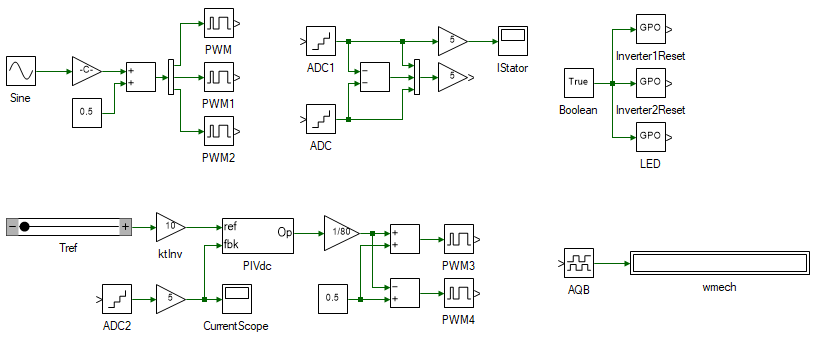
The bottom part of the model consists of a DC motor in current-control mode. The top section of the model consists of sine PWM that controls the induction motor's stator-voltage magnitude and frequency. To its right are the 3Φ current-measurement blocks. The phase-A and phase-C currents are measured. The phase-B current is computed using the fact that the sum of the 3Φ currents equals zero.
Open the properties of the slider tool, Tref. The torque is increased in steps of 0.01 Nm. The output of this block is scaled by the inverse motor torque constant, 1/k_T, and is then set as reference for the DC motor current control loop.

In the kTInv gain block next to the Tref slider, set the gain value to 1/k_T, using the k_T value obtained in the DC motor characterization experiment.
Open the IMParam script file and set the variable Vsrated to 25 and frated to 50.
Connect the induction motor to Inverter 1 (the color of each motor terminal must match that of the corresponding inverter terminal). Connect the DC generator to Inverter 2 (once again, the color of each motor terminal must match that of the corresponding inverter terminal).

Connect the three-inverter module to the DC power supply. Connect the three-inverter to the computer via USB. Connect the generator speed feedback to the three-inverter's Encoder 1 DSUB connector in the back panel.
Within the script file, set variable f to 30.
Turn ON the DC power supply and set the voltage to 40 V.
Ensure that the button on the top dock is pressed to enable real-time mode. Click the run button.

Run the model and note the steady-state speed for different loads. Change the load in steps of 0.01 Nm using the Tref slider, and record the rotor speed ω_mech in the table below.

T_l (Nm)	ω_mech (at f = 30 Hz)	slip	T_em (Nm)	ω_mech (at f = 40 Hz)	slip	T_em (Nm)	ω_mech (at f = 50 Hz)	slip	T_em (Nm)
0.0
⋮
0.06

Stop model data logging. Change the applied-voltage frequency in the script file to 40, rerun the model, and note the speed results for different load torques. Repeat the same process for f = 50.
Turn OFF the DC power supply.
In the table above, the electromagnetic torque is calculated using:
$T_{\mathrm{em}} = T_{l} + T_{c} + B\omega _{\mathrm{mech}}\tag{9}$
Slip is calculated using Eqns. 3 and 4.

This is the torque-slip characteristic of the induction motor, showing the relative drop in speed with increasing load torque. In the next part of the experiment, a closed-loop speed controller is implemented to maintain a constant speed as the load torque varies. The details of the controller design are part of the advanced electric drives lab and are not discussed here. For further reading, refer to Induction motor V/f control.

Real-time closed-loop torque-speed characteristic

Open Workbench and pin the Explorer and Properties docks.
Navigate to and open the IMSpeed project file in the Experiment8\ClosedLoop folder, usually found in the following location: C:\Program Files (x86)\Sciamble\WorkBench v1\Examples\CUSPLab\BasicDrives.
Expand the project and open the IMVbyF model file shown below:

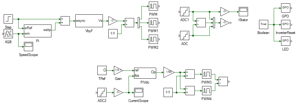
As before, the bottom part of the model consists of a DC motor in current-control mode. The top section of the model consists of closed-loop speed control, in which the applied stator-voltage frequency is increased or decreased using a PI controller based on the error between the desired and actual rotor speeds. The output-voltage magnitude is set based on Eqn. 7 so that, for a given stator-voltage frequency, the voltage magnitude generates the rated magnetizing current.
Turn ON the DC power supply and set the voltage to 40 V.
Ensure that the button on the top dock is pressed to enable real-time mode. Click the run button.
Vary the load torque using the Tref slider in the same 0.01 N·m steps used in the open-loop test, and record the steady-state rotor speed at each load torque.
Observe that the motor speed remains constant at steady state as the load torque changes.
Click the button to stop the model.
Turn OFF the DC power supply and disconnect all connections, including the USB cable.

This concludes the experiment on open-loop torque-speed/slip characterization of the induction motor and the introduction to its closed-loop speed control.

Lab report and reading assignment

Plot the result of T_em (y-axis) as a function of slip (x-axis).
Attach a plot of ω_m under open-loop speed control for all the different frequencies.
Did the motor stall, or did its speed become negative at a particular torque step? If so, why did this happen? If not, explain what would happen to the induction motor speed if the load torque were continuously increased.
Attach a plot of ω_m under closed-loop speed control.