


In this experiment, a mathematical model of a permanent-magnet DC motor will be simulated using the parameters estimated in the previous experiment. It will be shown that the motor speed cannot be held constant under varying load and voltage conditions. To overcome this, a closed-loop system will be developed using a PI controller so that the output speed closely matches the desired speed under various load conditions. Finally, the designed system will be run in real time to control the actual DC motor at a constant speed.
Motor model
The DC motor model characterized in the previous experiment is summarized in transfer-function form in Eqns. 1 through 4:
where
Va : terminal voltage
Ea : back-emf
Ia : armature current
Ra : armature resistance
La : armature inductance
ke : back-emf constant
kt : torque constant
J : rotor inertia
B : coefficient of viscous friction
Tc : torque due to Coulomb friction
Tem : output/electromagnetic torque
Tl : load torque
ωm : rotor speed
Depending on the application, the motor's output torque, speed, or position may need to be controlled. In the following section, a PI controller is designed to control the motor's output torque by controlling the applied terminal voltage.
Controller design
Consider a scenario in which the motor's output, or electromagnetic, torque must be controlled. Eqn. 2 shows that this can be achieved directly by controlling the motor armature current. This is accomplished using a proportional-integral (PI) controller whose transfer function is given in Eqn. 5, where ki,p and ki,i are the proportional and integral gains, respectively. The input to this controller, Ei, is the current error: the difference between the desired armature current Iref and the actual armature current Ia, as shown in Eqn. 6. The output of this controller is the armature voltage that must be applied to obtain the desired armature current and, in turn, the desired motor output torque.
The current-control system is summarized below, where M(s) is the actual motor model:
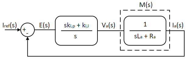
For a small change in the PI controller's error signal, the corresponding change in current, obtained from Eqns. 1, 5, and 6, is given below:
The back-emf term has been ignored in the small-signal model above because, when Va changes, Ia changes much faster than Ea. This is because the mechanical time constant of the motor, given by J/B, is much larger than the electrical time constant, given by La/Ra. Since the back-emf is proportional to the rotor speed, it responds more slowly than the armature current to a step change in the applied voltage and can therefore be ignored in the equation above. The overall small-signal model is obtained by combining the two equations above.
The ki,p and ki,i gain values are adjusted to obtain the desired transient response. There are multiple ways to quantify the desired response. In the time domain, the desired rise time and overshoot for a step input are usually specified, and the gains are adjusted to satisfy these requirements. Alternatively, in the frequency domain, the desired phase margin and crossover frequency are specified. We will use the latter approach because it provides a better picture of system stability. The steady-state response of the system is obtained by substituting s = jω into Eqn. 9.
The system above is tuned for a desired phase margin of Φi at the crossover frequency ωi,c as follows. At the crossover frequency, the system gain equals 1, and the system phase shift equals -π + Φi. Substituting this into Eqn. 10:
where
and
Given the desired Φi and ωi,c and the motor parameters, the PI gains can be solved using Eqns. 11 through 13.
The controller above maintains the motor at the desired current and, in turn, the desired motor torque while other system inputs vary. To achieve speed control rather than torque control, the system is modified by adding an outer speed PI controller to the existing inner current PI controller, as shown below:
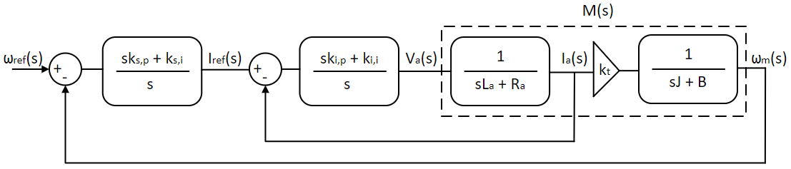
Here, M(s) is the actual motor model, and I(s) is the current-controlled system model, which includes the current PI controller and the motor's armature-current model.
To control the motor's speed rather than its torque, the same procedure can be followed with the following simplifying assumption: the response time of the motor current is an order of magnitude shorter than that of the motor speed for a step change in the applied voltage. This is achieved by setting the crossover frequency—which is also the system bandwidth in this case—of the current-loop PI controller an order of magnitude higher than that of the speed-loop PI controller. Thus, for a step change in the applied voltage, the current reaches its final steady state much earlier than the motor speed. Therefore, when tuning the speed controller, I(s) in the figure above can be assumed to be 1. The simplified speed controller model is shown below:
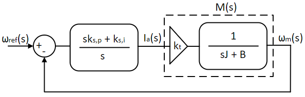
Let Es = ωref - ωm be the speed error. With the inner current loop approximated as unity, the open-loop transfer function from a small change in speed error to the resulting change in motor speed is:
The system above is similar to the current controller designed earlier. Following the same procedure gives the speed controller's gains:
where
and
where ks,p and ks,i are the speed PI controller's proportional and integral gains.
The above speed control model is simulated using Workbench in this section.
 Note
NoteSave the model at frequent steps.
Open-loop motor model
Create a new project and add a new model file to the project.
Set this model file as Start model/Function in the project properties.
Open the model properties and set Step time to 1E-4.
Drag and drop a subsystem tool from the Signal Routing tool class in the Toolbox.
A subsystem is an enclosure within which more tools can be added. Double-click the subsystem to open it.
Drag and drop the following tools from the Toolbox to the subsystem model and connect them as shown.
| # | Tool type | Tool class | Tool name |
|---|---|---|---|
| 1 | In-port | Signal Routing | I |
| 2 | Adder Subtractor | Math Block | Add |
| 3 | Transfer Function | Continuous | TransferFnc |
| 4 | Out-port | Signal Routing | O |
| 5 | Gain | Math Block | Gain |
| 6 | In-port | Signal Routing | I1 |
| 7 | Adder Subtractor | Math Block | Add1 |
| 8 | Transfer Function | Continuous | TransferFnc1 |
| 9 | Gain | Math Block | Gain1 |
| 10 | Out-port | Signal Routing | O1 |
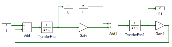
Change the properties of each tool to the values listed in the table below. The reason for each value is given in the rightmost column.
| Tool name | Property field | Property value | Comments |
|---|---|---|---|
| I | Name | Va | Motor applied terminal voltage Va |
| Add | Arithmetic operation | +- | Computes Va - Ea in Eqn. 1 |
| TransferFnc | Numerator | {1} | Numerator of transfer function in Eqn. 1 which is equal to 1. |
| TransferFnc | Denominator | {La, Ra} | Denominator of the transfer function in Eqn. 1. Substitute the values for La and Ra obtained from the previous experiment. The output of this tool is the motor current. |
| O | Name | Ia | This is the motor current. |
| Gain | Gain | kt | Substitute the value of kt = ke obtained from the previous experiment. The output of this tool is Tem, as given by Eqn. 2. |
| I1 | Name | Tl | Load torque |
| Add1 | Arithmetic operation | -+ | The differential torque in Eqn. 3 is the output of this tool, which computes Tem - Tl. For this model, Tc is ignored, but it may also be subtracted if desired. |
| TransferFnc1 | Numerator | {1} | Numerator of transfer function in Eqn. 3 which is equal to 1. |
| TransferFnc | Denominator | {J, B} | Denominator of the transfer function in Eqn. 3. Substitute the values for J and B obtained from the previous experiment. The output of this tool is the motor speed. |
| Gain1 | Gain | ke | The motor speed is scaled by ke to obtain back-emf Ea. This is looped back to Add to get the voltage difference. |
| O1 | Name | wm | This is the motor speed ωm. |
Return to the main motor model by clicking its tab at the top.
Resize the subsystem so that all the ports can be seen. A tool can be resized by clicking and dragging any of the four squares in the tool's corner.
To observe the motor speed and current when a voltage and load are applied to the motor, add the following tools to the main model and connect them as shown.
| # | Tool type | Tool class | Tool name |
|---|---|---|---|
| 1 | Step | Signal Sources | Step |
| 2 | Step | Signal Sources | Step1 |
| 3 | Mag-time Scope | Display | Scope |
| 4 | Mag-time Scope | Display | Scope1 |
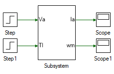
Change the properties of each tool to the values listed in the table below.
| Tool name | Property field | Property value | Comments |
|---|---|---|---|
| Step | Final value | 10 | Start at 0 V and step the applied voltage to 10 V |
| Step | Step time | 1 | Step the voltage at time t = 1 s |
| Step1 | Final value | 0.05 | Start at 0 Nm and step the load torque to 0.05 Nm |
| Step1 | Step time | 7 | Step the load at time t = 7 s |
Run the simulation model and observe the current and speed results in the scopes. As shown, the current and speed both change when either the applied voltage or the load torque is varied. In the following steps, the PI controller designed earlier is added to control the motor current and speed profiles.
Motor current control
In this section, the current through the motor is controlled using a PI controller.
Compute ki,p and ki,i using Eqns. 11 through 13 (first compute C1 using Eqn. 12, then ki,i using Eqn. 13, and finally ki,p using Eqn. 11) so that the system has a phase margin of Φi = π/3 at the crossover frequency ωi,c = 2π x 200. The crossover frequency is chosen as 200 Hz, which is sufficiently below the switching frequency of 6 kHz. This prevents the current controller from trying to compensate for the switching-current harmonics.
Delete the Step tool connected to the Va port of the motor model.
Add another subsystem to the model, in which the PI controller will be modeled. Double-click the subsystem to open it.
Drag and drop the following tools from the Toolbox to the subsystem model and connect them as shown.
| # | Tool type | Tool class | Tool name |
|---|---|---|---|
| 1 | In-port | Signal Routing | I |
| 2 | In-port | Signal Routing | I1 |
| 3 | Adder Subtractor | Math Block | Add |
| 4 | Gain | Math Block | Gain |
| 5 | Gain | Math Block | Gain1 |
| 6 | Integrator | Math Block | Integrator |
| 7 | Adder Subtractor | Math Block | Add1 |
| 8 | Saturation | Non-linear | Saturation |
| 9 | Out-port | Signal Routing | O |
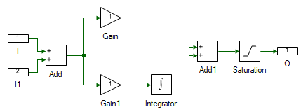
Change the properties of each tool to the values listed in the table below.
| Tool name | Property field | Property value | Comments |
|---|---|---|---|
| I | Name | Ref | Desired reference motor current. |
| I1 | Name | Fbk | Actual motor current. |
| Add | Arithmetic operation | +- | Difference between the desired and actual motor current. |
| Gain | Gain | ki,p | Substitute the value of ki,p computed in step 1. |
| Gain1 | Gain | ki,i | Substitute the value of ki,i computed in step 1. |
| Integrator | Integrator Type | Anti-windup | Reason explained later. |
| Integrator | Upper Limit | 38 | Set to the maximum positive output voltage. This is equal to the DC bus voltage minus the device drop (≈ 1.5 V). |
| Integrator | Lower Limit | -38 | Set to the minimum negative output voltage. This is the negative of the DC bus voltage minus the device drop (≈ 1.5 V). |
| Saturation | Upper Limit | 38 | Set to the maximum positive output voltage. This is equal to the DC bus voltage minus the device drop (≈ 1.5 V). |
| Saturation | Lower Limit | -38 | Set to the minimum negative output voltage. This is the negative of the DC bus voltage minus the device drop (≈ 1.5 V). |
| O | Name | Out | Applied terminal voltage to generate the desired current profile. |
When there is a large difference between the desired and actual currents, the PI controller produces a large output voltage to correct the error quickly. In a real-world system, the magnitude of this voltage is limited by either the available DC bus voltage or the voltage ratings of the motor and power electronics. Hence, in a practical implementation of a PI controller, the controller output is limited to the maximum possible voltage. During transient conditions, when the actual current differs from the desired current, the integrator in the PI controller rapidly builds its output to a large value because of the persistent input error. When the error returns to zero, this large integrator output does not decrease immediately and causes the actual current to overshoot the desired value. The resulting negative error causes the integrator output to fall, but it can fall by a much larger amount than desired, causing the current to undershoot. This process repeats, and the resulting oscillation dies down slowly. To avoid this, the range over which the integrator is active is clamped by setting it to Anti-windup. If the integrator output reaches this limit, the integrator is disabled until the polarity of the error reverses. This significantly improves the system response.
Return to the main motor model by clicking its tab at the top.
Resize the PI controller subsystem so that all the ports are visible.
Add a Step tool and connect the model as shown. Step the current to 1 A at t = 1 s by setting Final value to 1 and Step time to 1.
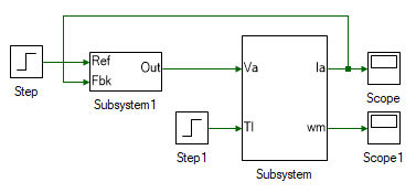
Run the simulation and observe the motor-current and speed results. In the current scope, zoom in at t = 1 s to view the step response. As shown, the current settles to the final value within a few milliseconds, whereas the speed takes a few seconds to settle to its final value. This justifies the earlier assumption in Eqn. 8, where the back-emf was ignored in the small-signal model because it changes much more slowly than the current. In most practical motors, the mechanical time constant is orders of magnitude higher than the electrical time constant.
Recompute ki,p and ki,i for Φi = π/6 and Φi = π/2, and obtain the current and speed responses for the computed gain values.
Motor speed control
In this section, the speed of the motor is controlled using a PI controller.
Compute ks,p and ks,i using Eqns. 14 through 17 so that the system has a phase margin of Φs = π/3 at the crossover frequency ωs,c = ωi,c/10 = 2π x 20. The crossover frequency is chosen as 20 Hz, which is one tenth of the crossover frequency of the inner current loop.
Remove the connection between the Step tool and the current PI controller subsystem.
Copy and paste (Ctrl + C, Ctrl + V) the current PI controller subsystem, as shown, to add a speed PI controller. Connect the tools as shown.
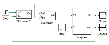
The reference speed is stepped to 100 rad/s at t = 1 s. To do this, change the Final value of the Step tool connected to the speed PI controller to 100 and Step time to 1.
Change the PI controller gain values in the pasted subsystem to the values computed in step #1.
Run the simulation and observe the speed. As shown, the speed settles rapidly to the desired speed compared with the open-loop system. The speed is also maintained when the load torque is applied. Contrast this with the open-loop case, in which the speed drops when a load torque is applied.
Observe the current result. The current profile will vary depending on the motor parameters and controller gain values used. In most cases, when used with the intended motor, the motor current would rise above 5 A, which is the maximum current limit of the three-inverter module. To prevent this overcurrent, the outputs of the integrator and PI controller must be limited, as was done for the current PI controller. In the speed PI controller, set Upper Limit to 5 and Lower Limit to -5 for both the Integrator and Saturation tools.
Rerun the simulation and observe the result.
NoteThe steady-state motor current and speed cannot both be controlled independently at the same time. The only quantity within the motor that the user can directly control is the applied terminal voltage. Thus, only one motor variable can be controlled at steady state: the motor current, rotor speed, or rotor position. In speed-control mode, the inner current loop merely dictates the path that the motor current takes to reach its final steady state. Its final value cannot be controlled independently.
In the previous section, the motor speed-control model was simulated. In this section, the same system is run in real time to control the speed of an actual motor.
Open a new Workbench session.
Create a new project and add a model file to it. Set this model file as the Start model/Function in project properties.
Open model properties and set the Step time to 0.0001 and Run time to 2.
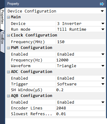
Within the project properties, select the drop-down menu at the top, and then select Device Configuration. Change the following properties:
Change Device within Main sub-division to 3 Inverter
Change Run Mode within Main sub-division to Till Runtime.
Change Frequency (Hz) within PWM Configuration sub-division to 12000.
Change Waveform within PWM Configuration sub-division to Triangle.
Change Encoder Lines within AQB Configuration sub-division to 2048.
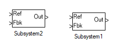
From the simulation model, copy and paste only the speed and current PI controllers, as shown:
Drag and drop the following tools from the Toolbox to the model and connect them as shown.
| # | Tool type | Tool class | Tool name |
|---|---|---|---|
| 1 | Step | Signal Sources | Step |
| 2 | AQB Speed | Hardware Integration | AQB |
| 3 | Mag-Time Scope | Display | Scope |
| 4 | Analog Input | Hardware Integration | ADC |
| 5 | Gain | Math Block | Gain |
| 6 | Mag-Time Scope | Display | Scope1 |
| 7 | Gain | Math Block | Gain1 |
| 8 | Constant | Signal Sources | Constant |
| 9 | Adder Subtractor | Math Block | Add |
| 10 | Adder Subtractor | Math Block | Add1 |
| 11 | PWM Output | Hardware Integration | PWM |
| 12 | PWM Output | Hardware Integration | PWM1 |
| 13 | True/False | Signal Sources | Boolean |
| 14 | Digital Output | Hardware Integration | GPO |
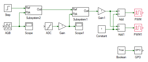
Change the properties of each tool to the values listed in the table below.
| Tool name | Property field | Property value | Comments |
|---|---|---|---|
| Step | Final value | 100 | Desired reference motor speed. |
| Step | Step Time | 1 | Step motor speed from rest to desired speed at time t = 1 s. |
| AQB | Channel | 1 | Actual motor speed feedback. |
| ADC | Channel | 3 | Actual motor current feedback. |
| Scope | Realtime log | Enabled | Enable to log real-time motor speed feedback. |
| Scope1 | Realtime log | Enabled | Enable to log real-time motor current feedback. |
| Gain | Gain | -5 | Scaling to convert ADC signal to actual current. The scaling value is given within the ADC property. |
| Gain1 | Gain | 1/80 | 1/(2 x Vdc), which converts the voltage to a value between ±0.5. |
| Constant | Magnitude | 0.5 | The signal above is centered at 0.5 to obtain the duty cycle. |
| Add1 | Arithmetic operation | -+ | The duty cycle of one inverter leg is obtained by adding the scaled duty to 0.5, and that of the other is obtained by subtracting it from 0.5. |
| PWM | Channel | 2 | Each PWM channel controls the voltage at one of the output terminals. |
| PWM1 | Channel | 1 | Each PWM channel controls the voltage at one of the output terminals. |
| Boolean | Value | True | This pulls the inverter out of reset so that it can be used to generate the desired output voltage. |
| GPO | Channel | 1 | The inverter being used is Inverter 1. |
Connect the motor (the one without the encoder) to Inverter 1 (the color of each motor terminal must match that of the corresponding inverter terminal). Even though the generator (the one with the encoder) is not used in this case, connect it to Inverter 2 instead of leaving the terminals open.
Connect the three-inverter module to the DC power supply. Connect the three-inverter to the computer via USB. Connect the generator speed feedback to the three-inverter's Encoder 1 DSUB connector in the back panel.
Turn ON the DC power supply and set the voltage to 40 V.
Ensure that the  button on the top dock is pressed to enable real-time mode. Click the run button.
Observe the speed and current results in the scopes. Click  to focus the results. After about 2 s, stop data logging by clicking
  .
.
Turn OFF the DC power supply.
In some cases, the current may be extremely choppy. This occurs because the speed controller tries to correct noise in the speed feedback in real-time mode. To avoid this, redesign the PI controller for a crossover frequency of 2 Hz, i.e., ωs,c = ωi,c/100 = 2π x 2.
Use the redesigned PI values and rerun the motor.
Replace the Step reference with a Sine reference whose Magnitude is 100 and whose Frequency is 1.
Turn ON the DC power supply and rerun the model.
Observe whether the motor tracks the reference speed.
Turn OFF the DC power supply and disconnect all the connections including the USB.
This concludes the experiment on DC motor speed control. In this experiment, the DC motor was actively loaded only in simulation, not in real time. This will be done in the following experiment, where the controller designed in this experiment will be used.
Attach plots of Ia and ωm from the simulation when the motor was operated in an open loop.
State the PI controller gain values obtained. Attach plots of Ia and ωm from the simulation when the motor was operated in current-control mode with different gain values.
State the PI controller gain values obtained. Attach plots of Ia and ωm from the simulation when the motor was operated in speed-control mode.
Attach a plot of ωm from real-time speed control.
In current-control mode, what would the speed profile look like if the friction coefficient B were zero and there were no voltage limitation?
How would you extend the speed-control model to perform position control? What system transfer function would be used to tune the PI controller?