Determination of Induction motor parameters

August 28, 2026
2 hours to complete
Workbench v1.5

Introduction

Like a DC motor, a 3Φ AC induction motor can be mathematically modeled as electrical and mechanical systems related by the relationships between back-emf and speed and between current and torque. In this experiment, the electrical and mechanical parameters of the induction motor are determined. These values are necessary to design a proper control system for the motor's speed, torque, or position.

Theoretical background

Motor model

Under steady-state operating conditions—i.e., when the motor speed, the magnitude and frequency of current and voltage, and the torque are constant—the induction motor can be modeled on a per-phase basis as a transformer, as shown below.

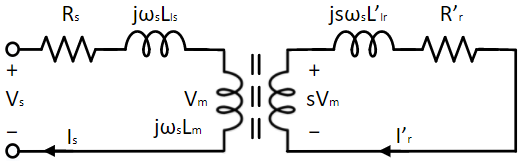
Induction motor steady-state equivalent circuit transformer model

The stator circuit is on the left, and the rotor circuit is on the right. They are electrically isolated by the air gap between the stator and rotor but are magnetically coupled. In a permanent-magnet synchronous motor, the rotor rotates at synchronous speed during steady-state operation:

\omega _{\mathrm{sync}} = \frac{2}{P} \times \omega _{s} = \frac{2}{P} \times 2\pi f_{s}\tag{1}

where P is the number of poles and f_s is the frequency of the applied voltage.

In the case of an induction motor, the rotor rotates at a speed slightly below the synchronous speed when operating in motoring mode:

\omega _{\mathrm{mech}} = (1 - s) \times \omega _{\mathrm{sync}}\tag{2}

where s is the motor slip and is typically between 0.005 and 0.05.

The voltage induced in the rotor is directly proportional to the motor slip and the stator voltage across the magnetizing inductance. If the rotor were stationary, i.e., ω_mech = 0, then the slip would be s = 1, and the circuit above would behave exactly like a transformer. When the rotor rotates at synchronous speed, i.e., ω_mech = ω_sync, the slip is s = 0, and no voltage is induced in the rotor because the rotor does not "see" any changing flux as it rotates at the same speed as the stator-induced air-gap flux. At any intermediate speed, the magnitude of the induced rotor voltage is proportional to the slip, and the frequency of the induced rotor voltage f_r is given by:

f_{r} = s \times f_{s}\tag{3}

The equation for the rotor circuit is given in Eqn. 4. It can be modified by canceling the slip on both sides, as shown in Eqn. 5.

s \times V_{m} = s \times \omega _{s}L_{m}I^{'}_{r} + R^{'}_{r}I^{'}_{r}\tag{4}

V_{m} = \omega _{s}L_{m}I^{'}_{r} + \frac{R^{'}_{r}}{s}I^{'}_{r}\tag{5}

This allows for further simplification of the equivalent circuit as shown below:

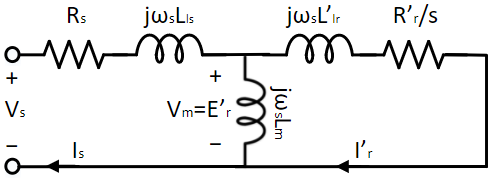
Induction motor steady-state equivalent circuit

The equivalent reflected rotor resistance $\frac{R^{'}_{r}}{s}$ in the equivalent circuit above consists of two components: the reflected rotor resistance $R^{'}_{r}$ and the mechanical-output equivalent resistance $R_{m} = R^{'}_{r}\frac{1-s}{s}$ . The power lost in R_m equals the output mechanical power given by:

P_{o} = \frac{3}{2} \times I^{2}_{r,\mathrm{peak}} \times R^{'}_{r} \times \frac{1 - s}{s} = T_{\mathrm{em}} \times \omega _{\mathrm{mech}}\tag{6}

where T_em is the motor's electromagnetic torque and I_r,peak is the peak rotor current.

The equivalent circuit modified to reflect the mechanical model, given by Eqn. 7, is shown below:

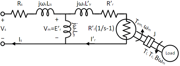
T_{\mathrm{em}} = T_{c} + B\omega _{\mathrm{mech}} + J\frac{d\omega _{\mathrm{mech}}}{dt}\tag{7}

Induction motor steady-state equivalent circuit with mechanical model

where

V_s : stator terminal phase voltage
R_s : per-phase stator resistance
L_ls : per-phase stator leakage inductance
L_m : per-phase magnetizing inductance
R^'_r : per-phase rotor equivalent resistance
L^'_lr : per-phase rotor equivalent leakage inductance
s : rotor slip
J : rotor inertia
B : coefficient of viscous friction
T_c : torque due to Coulomb friction
T_em : output/electromagnetic torque
T_l : load torque

In the following section, the motor parameters are determined by further simplifying the circuit under different operating conditions.

Parameter estimation

In this experiment, the electrical and mechanical model parameters are determined as follows:

R_s: Use a multimeter. The resistance measured across the two terminals is the line-to-line resistance. Divide it by 2 to obtain the per-phase resistance R_s. Alternatively, apply a constant voltage V_s of less than 2 V at the motor terminals and measure the steady-state stator current I_s. Divide V_s by I_s to obtain the line-line stator resistance, half of which gives the stator phase resistance R_s.
L_m: Apply the rated voltage V_s at the rated frequency f_s to the motor terminals. Under this condition, the motor should rotate with very low slip because there is no load torque other than the frictional component. Since the slip is small, the equivalent rotor resistance R^'_r/s is extremely large. Hence, the rotor can be considered open-circuited under no-load conditions. If the induction motor is coupled to a DC generator, a more precise estimate can be obtained by running the generator under speed control with the reference speed set to the synchronous speed. This essentially makes the slip s = 0, and thus the rotor is open circuited. From the stator current and voltage, the sum of magnetizing inductance and stator leakage inductance, L_s = L_m + L_ls, can be determined using the following equation:
$R^{2}_{s} + (L_{s} \times 2\pi f_{s})^{2} = \frac{V^{2}_{s,\mathrm{peak}}}{I^{2}_{s,\mathrm{peak}}}\tag{8}$
In a practical induction motor, L_m >> L_ls. Hence, the value obtained for L_s by solving the above equation can be reasonably approximated to be equal to L_m.
R^'_r, L_ls, and L^'_lr: Lock the rotor so that it does not rotate. Apply 25% of the rated frequency and gradually increase the applied voltage until the stator current reaches its rated value. The reason for choosing 25% of the rated frequency for this test is as follows. If a sufficiently high frequency is applied, the impedance of the magnetizing path is much higher than that of the rotor, i.e., ωL_m >> ωL_ls + R^'_r/s. Thus, the magnetizing-branch impedance can be ignored for this test. However, this frequency would not be representative of the actual motor, which under normal operation has rotor currents at a frequency close to the rated slip frequency. Consequently, the estimated resistance would be higher than the actual resistance because of the skin effect. If this test were performed at a very low frequency, close to the slip frequency, then the magnetizing impedance would not be sufficiently large relative to the rotor impedance to be ignored, which would complicate the estimation of the rotor parameters. Hence, to maintain the simplicity of the former approach and the precision of the latter, a frequency between the rated stator frequency and the rated slip frequency is chosen: f_s = 0.25 x f_rated. Under this condition, the equivalent circuit can be summarized as given by:
$(R_{s} + R^{'}_{r}) + j \times (L_{\mathrm{ls}} + L^{'}_{\mathrm{lr}}) \times 2\pi f_{s} = \frac{V_{s}}{I_{s}}\tag{9}$
Knowing the peak current I_s,peak, peak voltage V_s,peak, and phase shift Φ between the current and voltage, the leakage inductance and rotor resistance can be estimated as follows:
$R = R_{s} + R^{'}_{r}\tag{10}$ $L_{l} = L_{\mathrm{ls}} + L^{'}_{\mathrm{lr}}\tag{11}$ $\frac{2\pi f_{s} \times L_{l}}{R} = \tan(\Phi )\tag{12}$ $R^{2} + (L_{l} \times 2\pi f_{s})^{2} = \frac{V^{2}_{s,\mathrm{peak}}}{I^{2}_{s,\mathrm{peak}}}\tag{13}$
Solving these equations gives solutions for R and L_l, from which the leakage inductances and rotor resistance can be determined using Eqns. 14 through 16. The last two equations are empirical relations.
$R^{'}_{r} =R - R_{s}\tag{14}$ $L_{\mathrm{ls}} = \frac{2}{5}L_{l}\tag{15}$ $L^{'}_{\mathrm{lr}} = \frac{3}{5}L_{l}\tag{16}$
T_c and B: If the motor is not accelerating, i.e., its speed is constant, and no load is connected, the inertial-torque and load-torque components in Eqn. 7 become zero, leading to the following equation:
$T_{\mathrm{em}} = T_{c} + B\omega _{m}\tag{17}$
Apply a 3Φ voltage of magnitude V and frequency f, such that V/f = V_rated/f_rated, to the motor terminals. Measure the motor speed ω_m and peak stator current I_s,peak. The rotor peak current can be computed from the stator peak current using current division as given by Eqn. 18, where slip s is given by Eqn. 2. The electromagnetic torque T_em can be computed from the rotor peak current I_r,peak using Eqn. 6. Repeat the same process for different voltages and plot T_em (y-axis) versus ω_m (x-axis). The resulting plot will be linear. The slope of the plot equals the coefficient of viscous friction B, and the y-axis intercept is the frictional torque T_c due to Coulomb friction.
$I_{r,\mathrm{peak}} = I_{s,\mathrm{peak}} \times \frac{2\pi f_{s} \times L_{m}}{\sqrt{(2\pi f_{s} \times (L_{m} + L^{'}_{\mathrm{lr}}))^{2} + \left(\frac{R^{'}_{r}}{s}\right)^{2}}}\tag{18}$
J: Apply a 3Φ voltage of magnitude V and frequency f, such that V/f = V_rated/f_rated, to the motor terminals. Once the speed settles, measure the speed ω_m and peak stator current I_s,peak. At steady state, the electromagnetic torque T_em (Eqn. 7) solely compensates for drag due to friction. Disable the inverter so that the motor current dies down to zero rapidly. After this, there is no electromagnetic torque, and all the frictional losses must be supplied by the inertial energy. This causes the motor to stop gradually. This is summarized in Eqn. 19, which is obtained by setting T_em and load torque T_l in Eqn. 7 to zero.
$0 = T_{\mathrm{fric}} + J\frac{d\omega _{m}}{dt}\tag{19}$
At the moment the inverter is disabled, at time t = t_dis, the frictional-torque component T_fric is the same as the electromagnetic torque T_em(t_dis) just before the inverter is disabled, which can be computed using Eqns. 6 and 18. Substituting this into Eqn. 19 yields:
$J = -\frac{T_{\mathrm{em}}(t_{\mathrm{dis}})}{\frac{d\omega _{m}}{dt}(t_{\mathrm{dis}})}\tag{20}$ Thus, the motor inertia can be obtained by dividing the electromagnetic torque just before disabling the inverter by the motor deceleration just after disabling it.
Note
Disabling the inverter is not the same as actively setting its output voltage to zero. When the inverter is disabled, the stator current extinguishes much faster than the motor speed decreases, and the inertial energy is not returned to the source through the stator circuit. If zero terminal voltage were actively imposed instead, current could continue to flow, and some inertial energy would also be dissipated in the motor and inverter rather than only through friction.

Real-time parameter estimation

Assemble the induction motor–DC motor set as shown below:
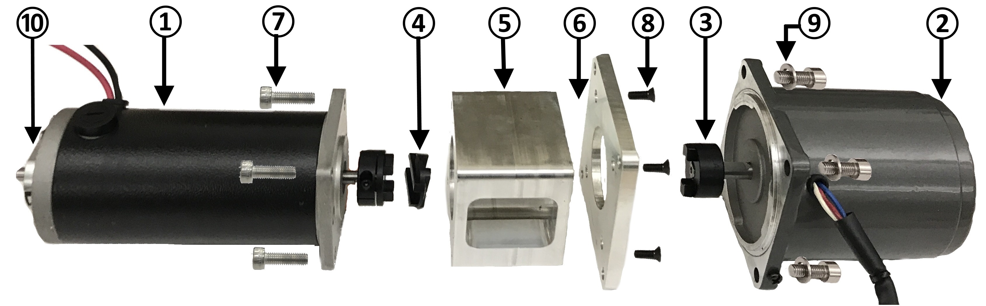
1. DC generator (the one with an A-quad-B encoder mounted on its back).
2. Four-pole induction motor.
3. Oldham coupler. Tighten if loose using M2.5 hex wrench.
4. Oldham coupling disk. Attach it to the motor and generator coupling.
5. Safety enclosure. The coupling unit resides inside the safety enclosure.
6. NEMA 34 to NEMA 23 frame converter plate.
7. M4 hex socket-head screws - 4.
8. M4 hex flat-head/socket-head screws - 4.
9. M5/M6 hex screws - 4.
10. 2048-line A-quad-B encoder. Attach the encoder cable to the A-quad-B encoder.
The wiring color code followed is:

DC (Inverter input):
1. DC +ve - ● (Red)
2. Ground - ● (Green)
3. ```
DC -ve  - ● (Black)
```
AC (Inverter output):
1. Phase A - ● (Black)
2. Phase B - ● (Red)
3. Phase C - ● (Blue)
The inverter output terminals are located on the front panel of the three-inverter module. Connect the induction motor terminals to the Inverter 1 terminals so that the colors of the corresponding terminals match. Connect the DC generator -ve (black terminal) to Inverter 2 A phase (black terminal) and DC generator +ve (red terminal) to Inverter 2 B phase (red terminal). Similarly connect the DC power supply to the inverter input, located on the back panel of the module.

Warning
Ensure that the DC power supply is turned off before making the connections. If the DC power supply does not have a dedicated ground terminal, that connection can be left floating. If present, it is strongly recommended that it be connected to the three-inverter module's ground terminal to mitigate any electrical hazard.
Connect the three-inverter to the computer via USB. Connect the generator speed feedback to the three-inverter's Encoder 1 DSUB connector in the back panel.

Note
For all computations in the steps below, the number of poles of the induction motor, P = 4.
R_s: Measure across the motor terminals using a multimeter. Divide the result by 2 to obtain the per-phase resistance.
L_m:
1. Open Workbench and pin the Explorer and Properties docks.
2. Navigate to and open the IMMotor project file in the Experiment7 folder, usually found in the following location: C:\Program Files (x86)\Sciamble\WorkBench v1\Examples\CUSPLab\BasicDrives.
3. Expand the project and open the IMElecEst model file by double-clicking the model node. Open the model properties by double-clicking anywhere in the blank space of the open model. Copy the value in the property labeled Name, which if previously unchanged will be IMElecEst.
4. Since this project has more than one model file, the project must be told which model to run. To do this, open the project properties by double-clicking the project node in the Explorer dock, and paste the copied model name (IMElecEst) into the Start model/Function field.
5. Shown below is the IMElecEst model:
  
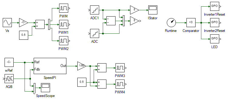
  The model consists of a DC motor speed controller that maintains the motor at synchronous speed. At the top is a 3Φ sine PWM block, which controls the applied terminal voltage and frequency. To its right are the 3Φ current-measurement blocks. The phase-A and phase-C currents are measured. The phase-B current is computed using the fact that the sum of the 3Φ currents equals zero.
6. Set the DC motor reference speed to π * IMParam:frated in the Constant block labeled wRef.
  
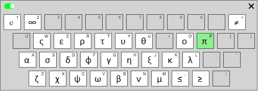
  To type the character π, click Alt+P. Pressing Alt will bring up the Greek keyboard.
7. Set the stator-voltage Magnitude to IMParam:Vsrated and Frequency to IMParam:frated in the Sine block labeled Vs. These values are defined in the IMParam script.
8. Turn ON the DC power supply and set the voltage to 40 V.
9. Ensure that the button on the top dock is pressed to enable real-time mode. Click the button.
10. Open the scope named IStator to see the data log of phase-A stator current. After about 5 s, stop the data logging by clicking on button. Automatically focus the scope result by clicking in the scope's toolbar.
11. Once the motor has reached steady state, zoom in on the peak of the stator current and note this value.
12. Compute the value of L_m using Eqn. 8, where V_s,peak can be obtained from the IMParam script file's Vsrated value.
R^'_r, L_ls, and L^'_lr:
1. Since this is a blocked rotor test, set the DC motor reference speed to 0 in the Constant block labeled wRef.
2. Set the stator-voltage Magnitude to IMParam:Vs and Frequency to IMParam:f in the Sine block labeled Vs. These values are defined in the IMParam script.
3. Open the IMParam file within the project and set the variable f to 15 and Vs to 5.
4. Turn ON the DC power supply and set the voltage to 40 V.
5. Ensure that the button on the top dock is pressed to enable real-time mode. Click the run button.
6. After about 5 s, turn off the DC power supply.
  
  Warning
  Do not let the test run continuously for more than 10 s. Since the stator current equals or exceeds the rated current, the motor tends to heat up quickly. In addition, the rotor is not rotating, which prevents the natural cooling provided by a rotating rotor. Therefore, turn off the DC power supply after every reading and turn it back on only when needed.
7. Open the stator phase-A current scope and observe the peak stator current at steady state. If the current is less than the rated current of 2.5 A, increase the induction motor stator voltage Vs in the IMParam script in small steps of 2 V.
  
  If the peak current is greater than the rated current, reduce the voltage in larger steps of 5 V to bring the current within the rated-current limit.
  
  Repeat this process until the peak current converges near the rated current.
8. Ensure that the DC power supply is turned off.
9. Once the motor has reached steady state, zoom in on the peak of the stator current and note this value.
10. Once the motor has reached steady state, zoom in on a zero crossing (a negative-to-positive transition) of the stator current. Note the time t_zc at which the zero crossing occurs. The number of stator-voltage cycles between t = 0 and t = t_zc is given by:
  $N = \operatorname{floor}((t_{\mathrm{zc}} \times f_{s}))\tag{21}$
  where f is the frequency of the applied voltage, and floor is the value rounded down to the nearest integer.
  
  From this, the phase shift between the stator current and voltage can be computed as follows:
  $\Phi = 2\pi \times (t_{\mathrm{zc}} \times f_{s} - N)\tag{22}$
11. Compute the values of R^'_r, L_ls, and L^'_lr from the phase shift and peak stator current using Eqns. 10 through 16.
12. Close the IMElecEst model.

T_c and B:

Both parameters are estimated using the same method in this step.

Open the IMBEst model within the same project.
Open the model properties and copy the Name property. Go to the project properties and set Start model/Function to the copied value.
Set the stator-voltage Magnitude to IMParam:Vs and Frequency to IMParam:f in the Sine block labeled Vs. These values are defined in the IMParam script.
Open the IMParam file within the project and set the variable f to 15 and Vs to f * Vsrated / frated.
Ensure that the button on the top dock is pressed to enable real-time mode. Click the run button.
After about 5 s, turn off the DC power supply.

Record the results in a table with the following layout:

V_s,peak (V)	I_s,peak (A)	ω_mech (rad/s)	I_r,peak (A)	P_o (W)	T_em (Nm)

where V_s,peak is the peak stator phase voltage, which can be obtained from the Magnitude property of the Sine block labeled Vs; I_s,peak is the peak stator current logged in the IStator scope; and ω_mech is the motor speed logged in the wmech scope. All these values must be measured after the motor reaches steady state following the application of the desired voltage. The remaining table entries are computed from these values using Eqns. 6 and 18.

Repeat the previous three steps for different motor frequencies f, from 15 Hz to 45 Hz in steps of 3 Hz. The voltage Vs in the IMParam script must always be maintained such that V/f = V_rated/f_rated.
Turn OFF the DC power supply and unplug the USB cable.
Plot T_em (y-axis) versus ω_mech (x-axis).

Measure the slope of the plot to estimate the coefficient of viscous friction B, and use the y-axis intercept to estimate the frictional torque due to Coulomb friction T_c.

J:
1. Open the IMJEst model within the same project.
2. Open the model properties and copy the Name property. Go to the project properties and set Start model/Function to the copied value.
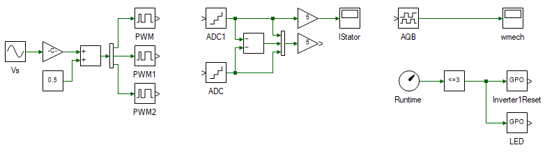
3. The model is shown below. The stator voltage is set to the motor's rated voltage IMParam:Vsrated and rated frequency IMParam:frated. Once the motor has reached steady state, the inverter is disabled at t = 3 s. This places the inverter terminals at high impedance so that the inertial energy is lost only through friction.
4. Reconnect the USB cable and turn on the DC power supply.
5. Ensure that is pressed. Click to run the model in real time.
6. Open the wmech scope to observe the motor speed. After data has been logged for 5 s, click to stop data logging. The results will look similar to the following:
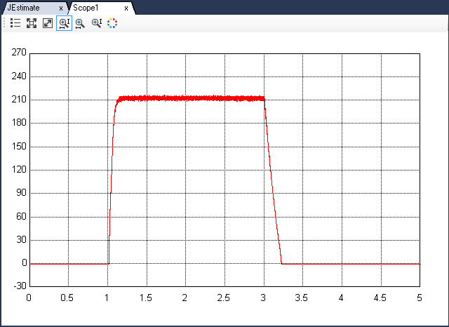
7. Zoom in on the speed at t = 3 s and determine the slope, as shown below.
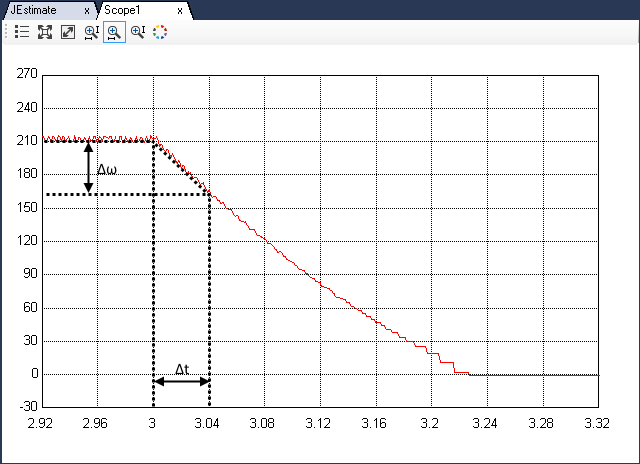
8. In the stator-current plot, note the current's peak magnitude just before the inverter is disabled at t = 3 s. Using this current, the speed, and the magnitude of the deceleration slope, calculate the inertia using Eqns. 6, 18, and 20.
Turn OFF the DC power supply and disconnect all the connections including the USB.

This concludes the experiment on induction motor characterization. The parameters estimated in this experiment will be used in the following experiments to tune a PI loop that controls the motor speed.

Lab report and reading assignment

Attach a plot of I_s from the L_m estimation.
Attach a plot of I_s from the R^'_r estimation.
Attach plots of I_s and ω_mech for different values of f from the B estimation.
Attach plots of I_s and ω_mech from the J estimation.
Attach the table from B estimation.
List the results of all final parameter values.